Scanning Tunneling Microscopy/Spectroscopy
The generalized tunneling current is: \(I_{t\to s}=-\frac{4\pi e}{\hbar}\int_{-\infty}^{+\infty}|M|^2\rho_s(\varepsilon)\rho_t(\varepsilon-eV)\cdot\left[f(\varepsilon-eV)-f(\varepsilon)\right]d\varepsilon\) Ignore the constant term: \(\begin{align} \mathcal{F}[I](k)&=\mathcal{F}[\rho_s](k)\cdot\mathcal{F}[\rho_t\cdot f](-k)-\mathcal{F}[\rho_s\cdot f](k)\cdot\mathcal{F}[\rho_t](-k)\\ \mathcal{F}[\rho_s](k)&=\frac{\mathcal{F}[I](k)+\mathcal{F}[\rho_s\cdot f](k)\cdot\mathcal{F}[\rho_t](-k)}{\mathcal{F}[\rho_t\cdot f](-k)} \end{align}\) The entanglement of $\rho_s$ and $f$ indicates the relation is not a simple convolution.
In the ultra-low temperature, the Fermi distribution degrades to the heaviside function $f(x) = \begin{cases} 1 &x\le 0
0 &x>0 \end{cases}$. Employing this we can get: \(I_{t\to s}=-\frac{4\pi e}{\hbar}|M|^2\int_{0}^{eV}\rho_s(\varepsilon)\rho_t(\varepsilon-eV)\relax\varepsilon\)
The measured DOS is: \(\begin{align} \frac{\mathrm{d}}{\mathrm{d}V}I_{t\to s}&=-\frac{4\pi e}{\hbar}\frac{\mathrm{d}}{\mathrm{d}V}\int_{-\infty}^{+\infty}|M|^2\rho_s(\varepsilon)\rho_t(\varepsilon-eV)\cdot\left[f(\varepsilon-eV)-f(\varepsilon)\right]d\varepsilon\\ &=-\frac{4\pi e}{\hbar}\int_{-\infty}^{+\infty}\left\{|M|^2\rho_s(\varepsilon)\frac{\mathrm{d}}{\mathrm{d}V}\rho_t(\varepsilon-eV)\cdot\left[f(\varepsilon-eV)-f(\varepsilon)\right]d\varepsilon+|M|^2\rho_s(\varepsilon)\rho_t(\varepsilon-eV)\cdot\left[\frac{\mathrm{d}}{\mathrm{d}V}f(\varepsilon-eV)\right]d\varepsilon\right\}\\ &=-\frac{4\pi e}{\hbar}\int_{-\infty}^{+\infty}\left\{|M|^2\rho_s(\varepsilon)\frac{\mathrm{d}}{\mathrm{d}V}\rho_t(\varepsilon-eV)\cdot\left[f(\varepsilon-eV)-f(\varepsilon)\right]d\varepsilon+|M|^2\rho_s(\varepsilon)\rho_t(\varepsilon-eV)\cdot\left[\delta(\varepsilon-eV)\right]d\varepsilon\right\}\\ &=-\frac{4\pi e}{\hbar}\int_{-\infty}^{+\infty}\left\{|M|^2\rho_s(\varepsilon)\frac{\mathrm{d}}{\mathrm{d}V}\rho_t(\varepsilon-eV)\cdot\left[f(\varepsilon-eV-f(\varepsilon))\right]d\varepsilon+|M|^2\rho_s(\varepsilon)\rho_t(\varepsilon-eV)\cdot\left[\delta(\varepsilon-eV)\right]d\varepsilon\right\}\\ &=-\frac{4\pi e}{\hbar}\left\{\int_{-\infty}^{+\infty}|M|^2\rho_s(\varepsilon)\frac{\mathrm{d}}{\mathrm{d}V}\rho_t(\varepsilon-eV)\cdot\left[f(\varepsilon-eV)-f(\varepsilon)\right]d\varepsilon+|M|^2\rho_s(eV)\rho_t(0)\right\}\\ &=-\frac{4\pi e}{\hbar}|M|^2\left\{\int_0^{eV}\rho_s(\varepsilon)\frac{\relax}{\relax V}\rho_t(\varepsilon-eV)\relax\varepsilon+\rho_s(eV)\rho_t(0)\right\} \end{align}\) The equation: \(\rho_t(0)\rho_s(eV)=-\frac{\hbar}{4\pi e|M|^2}\frac{\relax}{e\relax V}I(V)+\int_0^{eV}\rho_s(\varepsilon)\frac{\relax}{e\relax V}\rho_t(\varepsilon-eV)\relax\varepsilon\) It is a Type-2 Volterra equation, which has the form: \(y(t)=f(t)+\int_a^tK(t,x)y(x)\relax x, a=0 \text{ here}\) Here, \(y(x)\to\rho_s(\varepsilon),f(t) \to-\frac{\hbar}{4\pi e|M|^2\rho_t(0)}\frac{\relax}{e\relax V}I(V), K(t,x)\to\frac{1}{e\rho_t(0)}\frac{\relax}{\relax V}\rho_t(\varepsilon-eV)\) Since $\rho$ is even function, $\rho_t(\varepsilon-eV)=\rho_t(eV-\varepsilon)$, therefore, \(K(t,x)=K(t-x)\to -\frac{1}{e\rho_t(0)}\frac{\relax}{\relax V}\rho_t(eV-\varepsilon)\) Because for Laplace transformation $\mathcal{L}[K(t-x)]=e^{-sx}F_K(s)$. \(\begin{align} F_y(s)&=F_f(s)+\int_{0}^{\infty}e^{-st}dt\int_{0}^{t}y\left(x\right)K\left(t-x\right)\relax x\\ &=F_f(s)+\int_0^\infty y\left(x\right)\relax x\int_0^\infty K\left(t^{\prime}\right)e^{-st^{\prime}-sx}dt^{\prime},t'=t-x\\ &=F_f(s)+\mathcal{L}\left[K\left(t\right)\right]\cdot\mathcal{L}\left[y\left(t\right)\right]\\ F_y(s)&=\frac{F_f(s)}{1-F_K(s) } \end{align}\) Because $\rho_t(0)=0$, therefore: \(0=\frac{\hbar}{4\pi e|M|^2}\frac{\relax}{e\relax V}I(V)+\int_0^{eV}\rho_s(\varepsilon)\frac{\relax}{e\relax V}\rho_t(\varepsilon-eV)\relax\varepsilon\) Then: \(F_y(s) = -\frac{F_f(s)}{F_K(s)}\)
The Fourier transformation will give: \(\begin{align} -\frac{\hbar}{4\pi e |M|^2}\mathcal{F}\frac{\mathrm{d}}{\mathrm{d}V}I_{t\to s}&= \end{align}\)
Define $\rho_t’(\varepsilon-eV)=|M|^2\rho_t(\varepsilon-eV)\cdot\left[f(\varepsilon-eV)-f(\varepsilon)\right]$, def $\rho_t’‘(eV-\varepsilon)=\rho_t’(\varepsilon-eV)$, then $\rho_t’‘(x) = \rho_t’(-x)$ \(\begin{align} I_{t\to s}&=-\frac{4\pi e}{\hbar}\int_{-\infty}^{+\infty}\rho_s(\varepsilon)\rho_t'(\varepsilon-eV)\relax\varepsilon\\ &=-\frac{4\pi e}{\hbar}\int_{-\infty}^{+\infty}\rho_s(\varepsilon)\rho_t''(eV-\varepsilon)\relax\varepsilon\\ \mathcal{F}I_{t\to s}&=-\frac{4\pi e}{\hbar}\mathcal{F}\rho_s\cdot\mathcal{F}\rho_t'' \end{align}\)
SJTM: Scanned Josephson Tunneling Microscopy
Josephson Junction in STM
The most important properties between SJTM and SNS Josephson tunneling is the phase is unlocked and high frequency oscillation, leading to the unzero peak bias.[($\clubsuit$ TODO: Very important! A perspective. $\clubsuit$)]{style=”color: OliveGreen”}
The Josephson Juncion in STM is formed by the superconducting tip, the (surface) superconducting sample and the vaccumn barrier between them. Assuming the superconducting wave function on tip and sample are: \(\large\Psi_{\mathrm{s(t)}}=\sqrt{n_{\mathrm{SF,s(t)}}}\exp(-i\varphi_{\mathrm{s(t)}})\)
[($\clubsuit$ TODO: Using G-L minimal energy derivation, the other derivation is to be understood $\clubsuit$)]{style=”color: OliveGreen”}
When junction forms, the coupling energy is naive to be: \(F_J = -J\Psi_s^*\cdot\Psi_t+h.c.= -2J\sqrt{n_{\mathrm{SF,t}}n_{\mathrm{SF,s}}}\cos\Delta\phi\) Since the electric charge is the conservation charge of U(1) symmetry. There is a conjugation realtion between charge and phase: \(=i\) From the BCH formula, $e^{i\alpha q}f(\phi)e^{-i\alpha q}=f(\phi)+i\alpha[q,f(\phi)]+\dots$. With analogy to the Taylor expansion one can get $\frac{\partial f(\phi)}{\partial \phi}=i[q,f(\phi)]$. The current is defined by: \(\begin{align} \dot q &=-\frac{i}{\hbar}[H,q]\\ &=-\frac{1}{\hbar}\frac{\partial H}{\partial \phi}\\ I = -2e \dot q&=\frac{2eJ}{\hbar}\sin\Delta\phi=I_C\sin\Delta\phi\label{eq:josephsonrelation} \end{align}\) This is called Josephson relation.
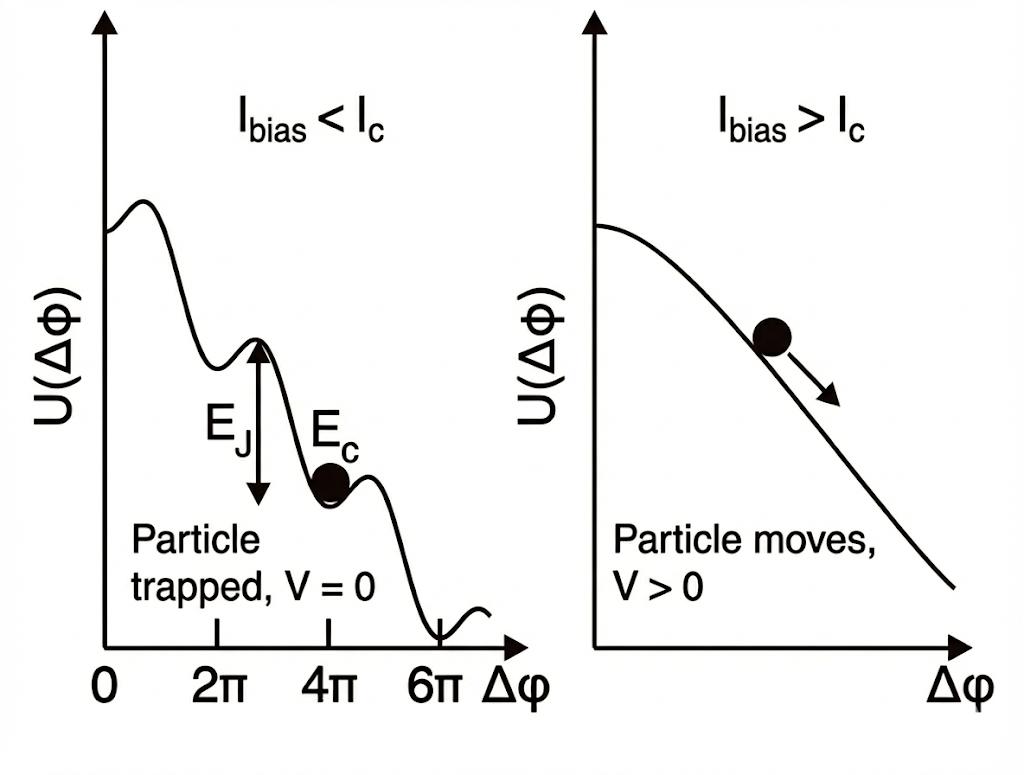
The full Hamiltonian describing the tunneling between tip and sample, including Capacitance, Josephson coupling, external current/bias, and the environment is: \(H_{\mathrm{total}}=\frac{\widehat{Q}^2}{2C}-E_J\cos\widehat{\phi}-\frac{\hbar I_{\mathrm{bias}}}{2e}\widehat{\phi}+Thermal+Env\label{eq:phaseH}\) It can be viewed as a particle $\phi$ with momentum $Q$ moving in a tilting wavy potential well. Starting from the phase-locked situations, applying for the typical SIS cases. In this case, the particle has low kinetic energy $E_C$, negligible compared to the ‘depth of well’ $E_J$. So when the ‘tilting’ $I_{bias}$ is not large enough, the particle is trapped in the bottom of the well, determining the voltage drop $V = \frac{\hbar}{2d}\dot\phi$ is zero. This reveals the reason why we observe the current at zero-bias in SIS Josephson junctions. When $I> I_C$, the potential well is disrupted $\dot V<=0$, so the I-V relationship back to normal. The discription can be viewed in the graph 1.
There are three energy scale in SJTM: charging energy $E_C$, Josephson energy $E_J$ and the thermal energy $E_T$. The charging energy is the energy of the capacitance: $E_C = \int U\mathrm d q=\int CU dU=\frac12CU^2=\frac{(2e)^2}{2C_J}$. $E_J$ is the josephson coupling energy mentioned above: $E_J = \frac{\hbar I_C}{2e}$. $E_T$ is $k_BT$ obviously.
The three energy scale have an estimated quantity:
Thermal energy: depends on the STM working temperature, varying from 20 mK to 4.3 K.
Capacitance: The maximum of capcitance is approximate $10^{-15}$ F. So the minimum of energy of capcitance is about 276 $\mu$eV $\approx$ 3.2 K.
Josephson coupling energy: suggested by Ambegaokar and Baratoff [@ambegaokar_tunneling_1963], the critical current has the relation in s-wave BCS superconductors: \(I_cR_N=\frac{\pi\operatorname{\Delta}(T)}{2e}\tanh{\left(\frac{\Delta(T)}{2k_BT}\right)}\) This leads to the result: \(E_\mathrm{J}=\frac{\pi\hbar}{4e^2}\frac{\Delta_\mathrm{CP}}{R_\mathrm{N}}\tanh\left(\frac{\Delta_\mathrm{CP}}{2k_\mathrm{B}T}\right).\) In a Josephson junction formed between an s-wave and an N-band superconductor, phase difference $\phi_i$ in Eq. ((eq:josephsonrelation)) is different among all bands. The critical current becomes a phase-sensitive sum: \(I_C = \sum_{i=1}^N I_{C,i}\cos\chi_i,\quad]chi_i=\phi_i-\phi_s\text{ under zero magnetic field}\) The critical current and resistance is described by the asymetric A-B formula: \(I_{\mathrm{C},i}R_{\mathrm{N},i}=\frac{2\Delta_\mathrm{T}|\bar{\Delta}_i|}{e\left(\Delta_\mathrm{T}+|\bar{\Delta}_i|\right)}K\left(\left|\frac{\Delta_\mathrm{T}-|\bar{\Delta}_i|}{\Delta_\mathrm{T}+|\bar{\Delta}_i|}\right|\right)\equiv\frac{\pi\Delta_{\mathrm{eff},i}}{2e},\)
Putting in the classical gap $\sim$ meV and effective resistance $\sim$ M$\Omega$ into the expression, the typical Josephson energy is about $3.5\mu$eV $\sim$ $40$mK[@cho_strongly_2019].
The quantitative relation among the three energy scale decides the model for the current spectrum:
RCSJ model: $E_T<E_J$, isolated from its electromagnetic environment.
Ivanchenko–Zil’Berman theory: $E_T>E_J$, the electromagnetic environment is Ohmic.
P(E), an arbitrary dissipative environment $Z(\omega)$ is present and $E_C>E_J$.
Ivanchenko–Zil’Berman theory
Taking thermal environment into consideration, the thermal energy gives the particle in (eq:phaseH) a hopping energy to jump over the wavy barrier, also serving as an Ohmic resistance, absorbing the energy difference in the cooper tunneling. Thinking the thermal fluactuation plays a role as random noise voltage $V(t)$, the resistance $R$ includes junction effective resistance and external resistance. The Kirchhoff laws shows the circuit should obey: \(\begin{align} I_c+I_j=I_{bias}&=\frac{(E+V(t))-V}{R}\\ \frac{E+V(t)-V}{R}&=C\frac{dV}{dt}+I_0\sin\varphi\\ C\frac{dV}{dt}+\frac{V}{R}+I_0\sin\varphi&=\frac{E+V(t)}{R}\\ C\left(\frac{\hbar}{2e}\ddot{\varphi}\right)+\frac{1}{R}\left(\frac{\hbar}{2e}\dot{\varphi}\right)+I_0\sin\varphi&=\frac{E+V(t)}{R}\\ C\ddot{\varphi}+\frac{\dot{\varphi}}{R}+\frac{2e}{\hbar}I_0\sin\varphi&=\frac{2e}{\hbar}\frac{E+V(t)}{R} \end{align}\) IZ first consider the particle is light like a feather, meaning $C\rightarrow0$, making it easier to be ‘pushed’. The equation turns into first-order Langevin equation, and the corresponding Fork-Plank equation is: \(\begin{align} \frac{d\varphi}{dt}=\underbrace{A(\varphi)}_\text{drift force}+\underbrace{\Gamma(t)}_\text{random noise}\\ \frac{\partial W}{\partial t}=\underbrace{-\frac{\partial}{\partial\varphi}[A(\varphi)W]}_{\text{ (Drift)}}+\underbrace{D\frac{\partial^2W}{\partial\varphi^2}}_{\text{ (Diffusion)}} \end{align}\) Here $A(\phi)={\frac{2e}{\hbar}E-\frac{2e}{\hbar}I_0R\sin\varphi},\Gamma(t)=\frac{2e}{\hbar R}V(t)$. Defining $\Omega_0=\frac{2eE}{\hbar},\Omega=\frac{2eI_0R}{\hbar}$. From the fluctuation-dissipation theorem, the thermal noise voltage satisfies: \(\langle V(t)V(t^{\prime})\rangle=2Rk_BT\delta(t-t^{\prime})\) So the diffusion term satisfies: \(\begin{gathered}\langle\Gamma(t)\Gamma(t^{\prime})\rangle=\left(\frac{2e}{\hbar R}\right)^2\langle V(t)V(t^{\prime})\rangle\\=\frac{4e^2}{\hbar^2R^2}\cdot(2R\Theta_0)\delta(t-t^{\prime})\\=2\left[\frac{4e^2\Theta_0}{\hbar^2R}\right]\delta(t-t^{\prime})\end{gathered}\) Take back to the FK equation we get: \(\frac{\partial W}{\partial t}=D\frac{\partial^2W}{\partial\varphi^2}+\Omega\cos\varphi W+(\Omega\sin\varphi-\Omega_0)\frac{\partial W}{\partial\varphi}\) Introduce the characteristic function: \(x_n(t)=\int_{-\infty}^{\infty}d\varphi e^{in\varphi}W(\varphi,t)\) The equation is processed as: \(\frac{\partial x_n}{\partial t}=(-Dn^2+in\Omega_0)x_n(t)-\frac{\Omega n}{2}[x_{n+1}(t)-x_{n-1}(t)]\) For the DC cases, we set $t\to \infty$. Partial differential term becomes zero. The difference equation leads to the Bessel function: \(x_n(\infty)=\frac{I_{n-iz_0}(z)}{I_{-iz_0}(z)}\) Using $\sin\varphi=\frac{e^{i\varphi}-e^{-i\varphi}}{2i}$, the I-V relation is: \(\begin{align} I &= \langle I_0\sin\varphi\rangle=I_0\frac{x_1(\infty)-x_{-1}(\infty)}{2i}\\ V&=\frac{\hbar}{2e}\langle\dot{\varphi}\rangle=\frac{\hbar}{2e}(\Omega_0-\Omega\ldots)\\ I(V)&=I_0\frac{1}{z}\frac{e^{\pi\delta}-e^{-\pi\delta}}{e^{\pi\delta}\int_0^{2\pi}e^{-z\cos x}e^{-\delta x}dx}, z=\frac{\Omega}{D}=\frac{E_J}{k_BT} \end{align}\) In very low thermal noise environment, the I(V) curve is: \(I=\frac{V}{R}\left(\sqrt{1+(\frac{I_0R}{V})^2}-1\right)\) This is the adjustment of RSJ model without noise. The more convincing case is $z\ll 1$ case: \(I=\frac{I_0z}{2}\frac{2eVD/\hbar}{(2eV/\hbar)^2+D^2}\) A more familiar form is: \(I(V)=\frac{1}{2}I_J^2Z\frac{V}{V^2+V_c^2}, Z\propto R,V_c\propto D\label{eq:IZ}\) The maximum Josephson current $I_m = \frac{Z}{4V_C}I_C^2$, $Z$ is the total electromagnetic impedance of all the elements and circuitry adjacent to the junction. Generally, the invariant gap will lead to a linear relationship of: \(I_{\mathrm{C}}\propto\sqrt{I_{\mathrm{m}}}\propto1/R_{\mathrm{N}},\label{eq:linearrelationship}\)
P(E) theory
If capacitance is small enough, making the ‘particle’ fly over the barrier without the assistance of thermal fluctuation. I(Z) model needs correction. In this case, thermal effect is neglected, and current is not a good quantum number. However, the task is to claim where the energy loss goes to.
In fact, the energy difference of cooper pair tunneling is absorbed by the environment, dissipation by photon emission actually. To describe the quantum fluctuation, we utilize Caldeira-Leggett model, which use infinity quantum oscillators to model the fluctuation: \(H=H_0+H_J=\sum_n\hbar\omega_n(a_n^\dagger a_n+\frac{1}{2})+\frac{\hat{Q}^2}{2C}-E_J\cos\hat{\phi}\) Treating $H_J$ as a pertubation term. The forward tunneling probability is: \(\Gamma(V)=\frac{2\pi}{\hbar}\sum_{i,f}\rho_i|\langle f|H_J|i\rangle|^2\delta(E_i-E_f+2eV)\) Here $|\langle f|-\frac{E_J}{2}e^{-i\hat{\phi}}|i\rangle|^2=\frac{E_J^2}{4}|\langle f|e^{-i\hat{\phi}}|i\rangle|^2$. Using the integral form of delta function: \(\Gamma(V)=\frac{E_J^2}{4\hbar^2}\int_{-\infty}^\infty dte^{i\frac{2eV}{\hbar}t}\underbrace{\langle e^{i\hat{\phi}(t)}e^{-i\hat{\phi}(0)}\rangle}_{\text{Phase Related}}\) Utilizing Baker-Campbell-Hausdorff formula and Gaussian approximation, we can define the core function $J(t)$: \(\langle e^{i\hat{\phi}(t)}e^{-i\hat{\phi}(0)}\rangle=\exp\left(\langle[\hat{\phi}(t)-\hat{\phi}(0)]\hat{\phi}(0)\rangle\right)\equiv e^{J(t)}\) Its Fourier transformation is the probability density of energy absorption $P(E)$: \(\mathbf{P(E)\equiv\frac{1}{2\pi\hbar}\int_{-\infty}^{\infty}dte^{J(t)}e^{\frac{i}{\hbar}Et}}\) Now it is clear to see the forward tunneling probability is $\Gamma(V)=\frac{\pi E_J^2}{2\hbar}P(2eV)$. Similarly we can get the backward probability, which means absorbing energy from external source to overcome the voltage drop. Combine them: \(I(V)=\frac{\pi E_J^2e}{\hbar}[P(2eV)-P(-2eV)]\label{eq:P(E)}\) To use this formula, we should know the form of $J(t)$. Usually, in the Temperature $T$ environment: \(J(t)=2\int_0^\infty\frac{d\omega}{\omega}\frac{\mathrm{Re}[Z_t(\omega)]}{R_Q}\left[\coth\left(\frac{\hbar\omega}{2k_BT}\right)(\cos\omega t-1)-i\sin\omega t\right]\) where $R_Q=\frac{h}{4e^2}\approx6.45k\Omega$, $Z_t(\omega)=\left(i\omega C+Z_{ext}^{-1}(\omega)\right)^{-1}$.
Current-bias SJTM
Notce that the I-V curve described by (eq:P(E))) and (eq:IZ) forbid non-zero current at zero-bias. This is the nature of phase-diffusion cases.
The following content is subtracted from the reference[@trahms_diode_nodate].
The SJTM is formed between Pb tip and Pb surface, doted by single Pb, Cr, and Mn. To reach RSJ/RCSJ phase, the contact between tip and sample must be very close. In this article, 50$\mu S$ conductance is reached at bias 10mV, which means current is about 500nA. To compare with this, the quantum conductance is about 77.48$\mu S$, corresponding to the zero-contact point. Rough caculation reveals the distance is about 0.19Å.
To achieve current-biased controller, a massive resistance $\sim1 M\Omega$ is in series with the junction. It is convincing the resistance makes major contributions to the whole junction, which makes the SJTM current-biased. The I(V) curve is obtained by changing the current/ voltage indeed.
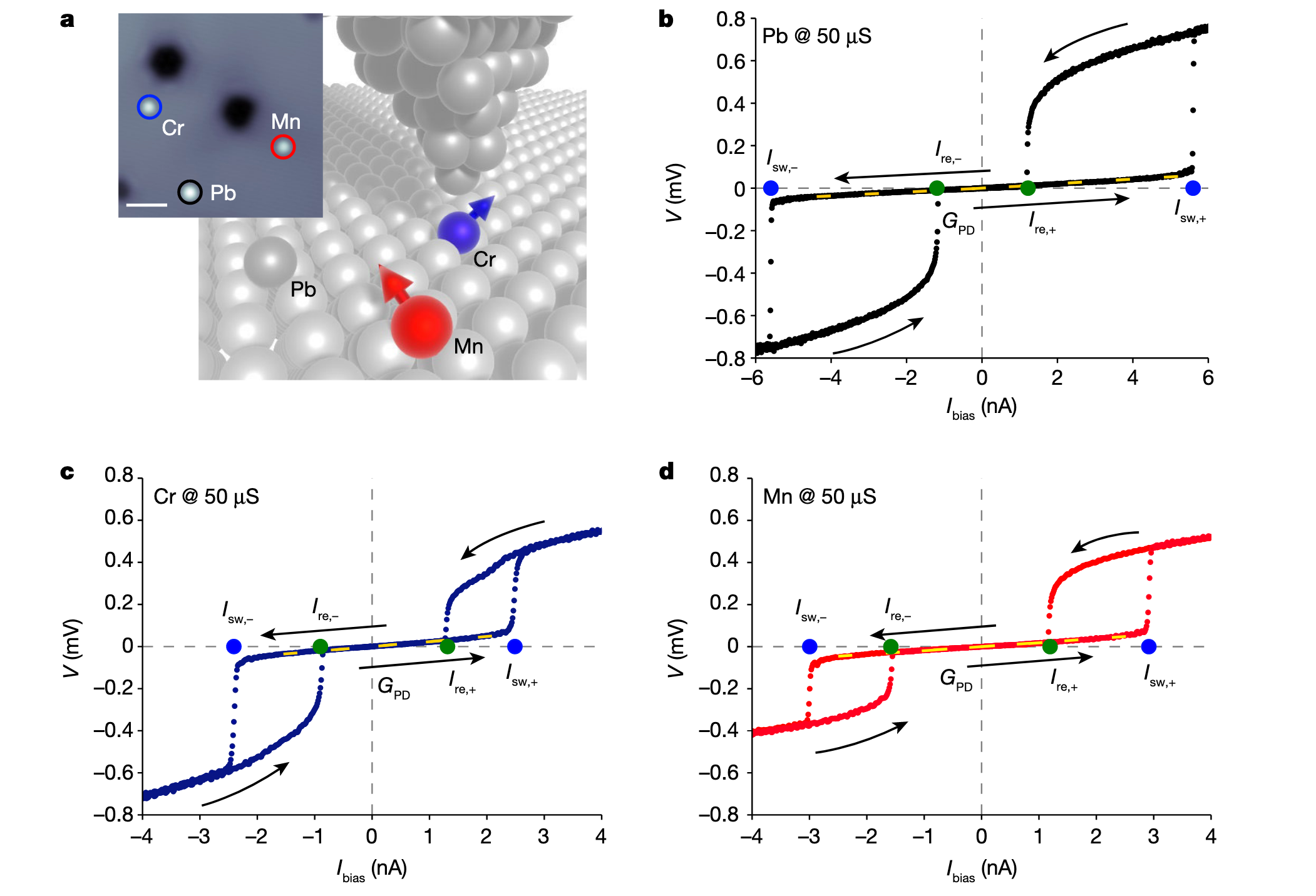
In 2, one can find out the common aysmmetry between retrapping current $I_{re}$ and switching current $I_{sw}$, the former means the particle in dissipation state, or so-called ‘run state’ with $V=\braket{\dot\phi}\neq0$, is trapped by the wavy potential. The latter is the DC Josephson current reaches the maximum and the particle rolled downwards. It is simple to imagine: In SJTM, the capacitance is roughly $\propto 1/d$. In this case, capacitance is very huge (thus in RCSJ regime). The phase particle is so heavy that it needs a quite deep well to trap a running one, making $I_{re}<I_{sw}$. However $I_{sw}\ll I_c\approx 107$nA revealing the important role of Nyquist noise.
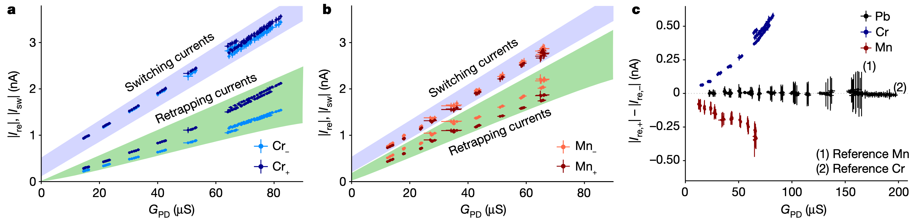
The more interesting is the asymmetry between the $I_{sw}^+$ and $I_{sw}^-$, $I_{re}^+$ and $I_{re}^-$ . They conduct IV data collection at different conductance (at same bias 10meV), obtaining averaged $I_{sw}$ and $I_{re}$. From the graph 3, first we can find out the $I_{re}$ and $I_{sw}$ are both linear to the conductance, which is align with the A-B formula $I_J\propto G$ ( very different from the scenario in multi-band cases!). Second, the asymmetry of $I_{re}$ is much larger than $I_{sw}$, which rull out the possible origin of asymmetry: asymmetric phase-current relation ($I\neq I_c\sin\phi$) .
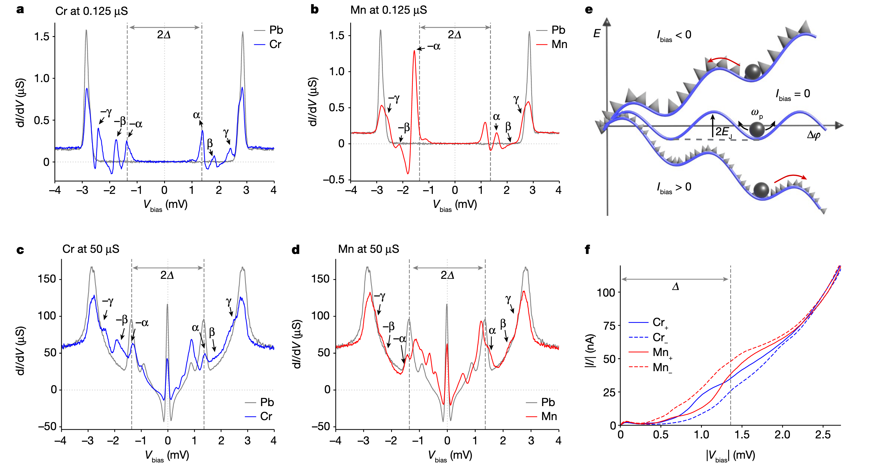
They then conduct the voltage-bias analysis. In low conductance regime (single quasi-particle tunneling regime) they identify Yu-Shiba-Rusinov state from the in-gap peaks ( in 50$\mu$S conductance, the in-gap peaks smear.). YSR state orginates from the magnetic impurities scatters the cooper-pair and breaks the pairing, can be obtained from the Anderson impurtiy model. The interacting Hamiltonian is: \(H_{\mathrm{int}}=\sum_{\mathbf{k},\mathbf{k}^{\prime}}\sum_{\sigma,\sigma^{\prime}}\psi_{\mathbf{k},\sigma}^{\dagger}[J\mathbf{S}\cdot\mathbf{s}_{\sigma,\sigma^{\prime}}+K\delta_{\sigma,\sigma^{\prime}}]\psi_{\mathbf{k}^{\prime},\sigma^{\prime}}.\) where $J=|t|^2\left{\frac{1}{|\epsilon|}+\frac{1}{\epsilon+U}\right},K=|t|^2\left{\frac{1}{|\epsilon|}-\frac{1}{\epsilon+U}\right}.$ A standard calculation can show that non-zero $K$ can induce the particle-hole asymmetry.
The important characteristics of the STS spectrum is that the asymmetry of height of the YSR pair state, though their bias positions are symmetric. This is the evidence that YSR breaking the particle-hole symmetry. Another evidence is shown in 4f, where they subtract the quasiparticle tunneling current $I_{qp}$ from the whole current curve. They point out the $I_{qp}$ is asymmetry between positive bias and negative bias regime, originating from the PHSB.
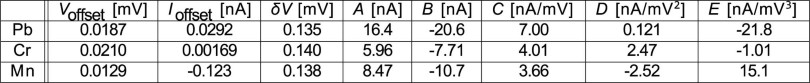
It is worth noting that, the current consist $I_{qp}, I_J, and \quad I_{bias}$. The subtraction is based on fitting: \(\begin{align} I_{\mathrm{meas}}(V)&=I_{\mathrm{j}}(V+V_{\mathrm{offset}})+I_{\mathrm{qp},0}(V+V_{\mathrm{offset}})+I_{\mathrm{offset}},\\I_{\mathrm{j}}(V)&=A\frac{V\delta V}{V^2+\delta V^2}+B\frac{V^3\delta V}{\left(V^2+\delta V^2\right)^2},\\I_{\mathrm{qp},0}(V)&=CV+DV^2+EV^3, \end{align}\) In the Extended Table of [@trahms_diode_nodate], the parameters are calculate by fitting:
The reconstructed I-V curve is presented in Fig.6. We can see the original I-V curve acts like thermal fluctuation dominated IZ model, even though the measurement condition is the same as 2 at 50 $\mu$S conductance. This reveals the importance of current-bias, which can control the $\phi$ position, while voltage bias can only control the averaged moving speed.

The article then claim the $I_{qp}$ plays a role of damping force (modifing the resisitance). Though the resistance $R_n$ of the Josephson junctions usually are the normal state resistance. For the junciton dynamics, we notice the retrapping occurs in gap, and the YSR induced current opens another channel besides the Ohmic channel, equivalent to a resistance in parallel, decreasing the effective resistance and damping the phase particle. The asymmetry of $I_{qp}$ leads to the asymmetry of the retrapping.
Solid Physics
The definition of classical superconductivity is about:
The transition temperature $T_c$ is a small fraction of Fermi temperature $T_F$.
We use conventional theory to describe the normal states.
No other phase change at superconductivity transition.
Conventional symmetry of Cooper pairs, for example, the translation symmetry in crystal and s-wave in orbital.
Phonons are exploited to transfer energy inside Cooper pairs.
Most behave like type-1 material, which only contains two states without a zero-resistant state but has an inner magnetic field.
The normal state
A normal state exists at the order of room temperature and below. Sommerfeld, Bloch, Landau, and Silin’s theorem can be used here.
Sommerfeld Model
The very simplest model of the normal state of a metal is Sommerfeld model. Sommerfeld model is based on the Drude model, which assumes:
Independent electrons assumption.
Free elections assumption and Fixed ions assumption.
View electrons as waves so that they will not collide with each other.
Fermi-Dirac statistics.
In this model, a single-particle eigenstate is a plane wave: \(\psi_k(r) = \frac{1}{\sqrt{\Omega}}e^{i\mathbf{k}\cdot\mathbf{r}}\) The energy is: \(\epsilon_k = \frac{\hbar k^2}{2m}\quad k=\frac{m \pi}{L}, m\in\mathbb{N}\) Fermi distribution gives out the average particle number on an eigenstate with energy $\epsilon_k$: \(f(\mathbf{k},\sigma)=\frac{1}{\exp{\frac{\epsilon-\mu}{k_BT}}+1}\) At zero temperature, the distribution reduces to the Heaviside function: \(f = \Theta(\mu-\epsilon_k)\quad k_F = (3\pi^2n)^{\frac{1}{3}}\) To prove the second equation: \(\begin{align} D(\epsilon) &=2\frac{2\pi V}{h^3}(2m)^{\frac{3}{2}}\epsilon^{\frac{1}{2}}\\ N &= \int_0^\infty f(\epsilon)D(\epsilon)\relax\epsilon\\ &=2\int_0^{E_F}\frac{2\pi V}{h^3}(2m)^{\frac{3}{2}}\epsilon^{\frac{1}{2}}\relax\epsilon\\ &=2\frac{2\pi V}{h^3}(2m)^{\frac{3}{2}}\frac{2}{3}E_F^{\frac{3}{2}}\\ \therefore k_F &= \frac{p_F}{\hbar}\\ &=\frac{1}{\hbar}\sqrt{2 m E_F}\\ &=\frac{1}{\hbar}\sqrt{2 m (\frac{3h^3n}{8\pi(2m)^{\frac{3}{2}}})^{\frac{2}{3}}}\\ &=\frac{1}{\hbar}(\frac{3h^3n}{8\pi})^{\frac{1}{3}}\\ &=(3\pi^2n)^{\frac{1}{3}} \end{align}\) In the case $T\neq 0$, but $T\ll T_F$. The distribution is slightly different from the step function. We can assume only states which is in an energy shell of width $\sim k_BT$ around the Fermi energy is different. In this case, the density of state (DoS) is defined to describe a state. From Sommerfeld model we know: $n\sim E_F^{\frac{3}{2}}$. Therefore, $\frac{\relax n}{\relax\epsilon}=\frac{3n}{2\epsilon_F}$. And: \(\begin{align} \chi_\mathrm{s}&=\mu_\mathrm{B}^2\frac{\relax n}{\relax\epsilon}\\ c_V&=\frac{\pi^2}3k_\text{B}^2T\frac{\relax n}{\relax\epsilon}\\ \sigma&=\frac13v_\mathrm{F}^2\frac{\relax n}{\relax\epsilon}\tau \end{align}\) [($\clubsuit$ TODO: How to prove? $\clubsuit$)]{style=”color: OliveGreen”}
Bloch Model
The Bloch model begins by using the Bloch wave to define a single-particle eigenstate: \(\psi_{\boldsymbol{k}n}(\boldsymbol{r})=u_{\boldsymbol{k}n}(\boldsymbol{r})e^{i\boldsymbol{k}\cdot\boldsymbol{r}}\)
Landau-Silin theory
In this theory, phenomenological interactions between conduction electrons including interactions induced by exchange of virtual lattice vibrations are considered.
This model introduces quasiparticles, which may be thought of intuitively as a real electron accompanied by a “dressing cloud” of other electrons and phonons.
Braid Group
Thinking about a model like:
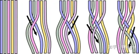
This model is composed of several tied braids, obeying the rules:
Each string is supposed to connect from one of the ends (called A) to the other end (called B).
Each string travels in one direction and any backward operation anywhere is not allowed.
All the strings can be seen as an evolution from an initial state to a final state. Braiding the strings like exchanging the adjacent ends and making nods will introduce much more information then initial states and final states, as the exchange operations are not topologically trivial. All the braiding operations make up a group called the braid group.
Take $B_4$ as an example. $B_4$ is based on four strings. Obviously, all braiding operations can be built up with three generators, like below:
\(\sigma_i\) is an operation which connects \(i\)th end to \(i+1\)th end, and the string start from \(i\)th end is beneath the string from \(i+1\)th. Just like anyons, the operation which makes the string travel across the string is topologically in-equilibrium to the previous, which is denoted as \(\sigma_i^{-1}\).
Let’s make a more generalized formation. Artin Braid group $B_n$ is composed of $n-1$ generators with a braid relations:
$\forall i-j \ge2\quad\sigma_i\sigma_j=\sigma_j\sigma_i$ - $\forall 1\ll i\ll n-1\quad \sigma_i\sigma_{i+1}\sigma_i=\sigma_{i+1}\sigma_{i}\sigma_{i+1}$
Here is a diagram that can illustrate the physical mean of braid relations:
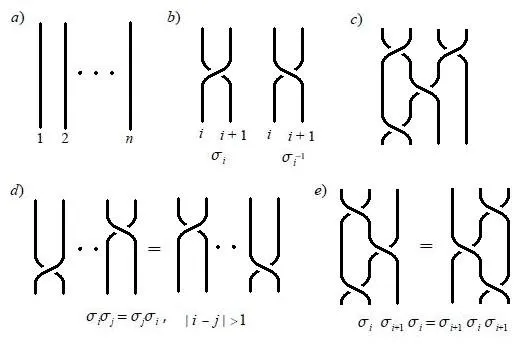
In a word, the equivalent of two juxtapositions means each initial state in both of them evolves in a same (across or beneath) way to the same final state.
Compared to the permutation group $S_N$, $B_N$ does not preserve $\sigma_i^2=1$, which corresponds to the anyonic statistics. This also results in the infinite size of $B_N$ ($S_N$ has a finite size of $N!$. The richness of the braid group is the key fact enabling quantum computation through quasiparticle braiding.
Majorana Fermion
Begin with Dirac Equation: \(\label{eq:DiracEquation} \left( i \gamma^\mu \partial_\mu - m \right) \psi = 0\) The Dirac matrices $\gamma^\mu$ satisfy the Clifford algebra: \(\label{eq:CliffordAlgebra} \left\{ \gamma^\mu, \gamma^\nu \right\} = 2 g^{\mu \nu} \mathbb{I}\) This is necessary to ensure the description obeys energy-momentum relation $E^2 = \bm{p}^2 + m^2$1. Another hidden property is: \(\gamma^0\gamma^\mu\gamma^0=\gamma^{\mu\dagger} \label{eq:3.3}\) This can be seen in the analogy to the Schrodinger equation, which implies a Hamiltonian $\gamma^0(\gamma^i p_i + m)$. If we want the Hamiltonian to be Hermitian, we need this relation.
There are several solutions to the Dirac matrices, which are called the Dirac matrices in different representations. If you want to study chirality, Weyl representation is the best choice. If you want to relate the Dirac equation to the Schrodinger Equation in Electromagnetic, Dirac representation is preferred. In this note, we will focus on another representation, called Majorana representation.
The motivation for Majorana’s representation is to find a pure real the formalism of the Dirac equation, this means the Dirac matrices should be pure imaginary. The representation is: \(\begin{align} \gamma^0=\begin{pmatrix} 0 & \sigma^2 \\ \sigma^2 & 0 \end{pmatrix}\quad \gamma^1=\begin{pmatrix} i\sigma^1 & 0 \\ 0 & i\sigma^1 \end{pmatrix}\\ \gamma^2=\begin{pmatrix} 0&\sigma^2\\ -\sigma^2&0 \end{pmatrix}\quad \gamma^3=\begin{pmatrix} i\sigma^3&0\\ 0&i\sigma^3 \end{pmatrix} \end{align}\) where the $\sigma^i$ are the Pauli matrices. The Dirac equation is built up by such matrices enables us to find a real solution $\psi$.
However, Majorana representation is not unique in any sense. There are infinitely many choices of the Dirac matrices which satisfy (eq:CliffordAlgebra) and (eq:3.3). An important theorem says that if there are two choices of Dirac matrices, both satisfying (eq:CliffordAlgebra) and (eq:3.3), they will be related by a similarity transformation involving a unitary matrix. In other words, the general solution of (eq:CliffordAlgebra) and (eq:3.3) can be obtained from the Majorana representation as: \(\Tilde{\gamma}^\mu=U^{\dagger}\gamma^\mu U\) where U is a unitary matrix. Then for a Majorna solution to the Dirac equation $\psi$, a general solution in any representation is: \(\Tilde{\psi}=U^{\dagger}\psi\) If the new solution is still Majorana field, it satisfy: \(U^{\dagger}\psi=(U^{\dagger}\psi)^*\) or \(\psi = UU^T\psi^*\) Note that since U is unitary, the combination $UU^T$ is also unitary. Instead of using U directly, it is customary to use another unitary matrix C which is defined by: \(\hat \psi=\gamma^0C\psi^*\) Than in a general representation, a Majorana fermion field satisfy: \(\psi = \hat\psi=\gamma^0C\psi^*\) Interestingly, $\hat\psi$ can be proved as the charge conjugation of $\psi$. This is commonly stated as the anti-Majorana fermion is itself.
Anyons
In physics, the exchange of two identical particles will not change our observation of the system, which means the probability will be invariant. This leaves a phase factor $e^{i\theta}$ to the wave function. And also, double exchange is equivalent to the origin. So we have: \(\begin{align} \Psi(\bm{r}_1,\bm{r}_2)&=e^{i\theta}\Psi(\bm{r}_2,\bm{r}_1)\\ \Psi(\bm{r}_1,\bm{r}_2)&=e^{2i\theta}\Psi(\bm{r}_1,\bm{r}_2)\\ \therefore e^{2i\theta}&=1\Rightarrow e^{i\theta}=\pm 1 \end{align}\) For bosons, the phase factor is $+1$, and for fermions, the phase factor is $-1$. However, if our consideration is limited to 2-dimensional space, the phase factor can be any value and anyons emerge.
![Anyon[@simula_quantised_2019]](/assets/img/notes/anyon.png)
In 3-dimensional space, any closed path $C$ is topologically equivalent to a single point, whether it includes a particle or not. This means that the path can be continuously deformed to a point without breaking. Recall that if we exchange two identical particles like c-part in Fig. 9, the operation is equivalent to a closed loop of one of them. The rotation of the reference point $p$ around the particle is equivalent to a closed loop of the particle around the reference point. So the exchange of two identical particles is topologically equivalent to the origin. However, in 2-dimensional space, the continuous deformation of a closed path to a point is interrupted by the particle’s existence. Describing such a system requires a nontrivial phase factor, which generally may take any value $\theta\in\left[0,2\pi\right]$.
The motivation to study anyons is to study electromagnetic in the (2+1)D system. In the (3+1)D Boltzmann system, all trajectories are distinguishable so that we can deform them into pure time component. In (3+1)D Bose or Fermi system, the statistics are just the correspondence of permutation group, as their trajectories can be separated. However, in the (2+1)D system, all trajectories can be topologically nontrivial as we move a particle around another.
This also gives rise to the relationship with the braid group. The topological classes of trajectories which take these particles from initial positions $R_1, R_2,\dots, R_N$ at time ti to final positions $R_1, R_2,\dots, R_N$ at time tf are in one-to-one correspondence with the elements of the braid group $B_N$. In the view of exchange statistics, the string passing over another $\sigma_i$ or under another $\sigma_i^{-1}$ corresponds to a clockwise or counter-clockwise exchange. The previous requirement that any intermediate time slice must intersect N strands,i.e., strands cannot “double back”, physically means no creation and annihilation halfway (as anti-particle evolves backward).
Topological properties of anyons
To fully describe the topology of anyons, we need the following characteristics:
The particle species.
The fusion rules $N_{ab}^c$.
$F$ matrix.
$R$ matrix.
Topological spin.
$S$ matrix.
Particle Species
The particle is characterized by its topological statistics. For example, Abelian anyons correspond to the 1D representation of the braid group, which means a phase $2\theta_{ab}$ is generated when braiding a particle of type A around a particle of type B. For non-Abelian anyons, which are associated with higher-dimensional representations of the braid group occurring when there is a degenerate set of $g$ states with particles at fixed positions $R_1, R_2, \dots, R_n$, the order of exchange matters. An element of the braid group, which exchanges particles 1 and 2—is represented by a $g\times g$ unitary matrix $\rho(\sigma)$ acting on these states, i.e.: \(\psi_\beta = [\rho(\sigma_1)]_{\alpha\beta}\psi_\beta\) The non-Abelian property is mathematically shown: \(\neq0\Leftrightarrow [\rho(\sigma_1)]_{\alpha\beta}[\rho(\sigma_2)]_{\beta\gamma}\neq[\rho(\sigma_2)]_{\alpha\beta}[\rho(\sigma_1)]_{\beta\gamma}\)
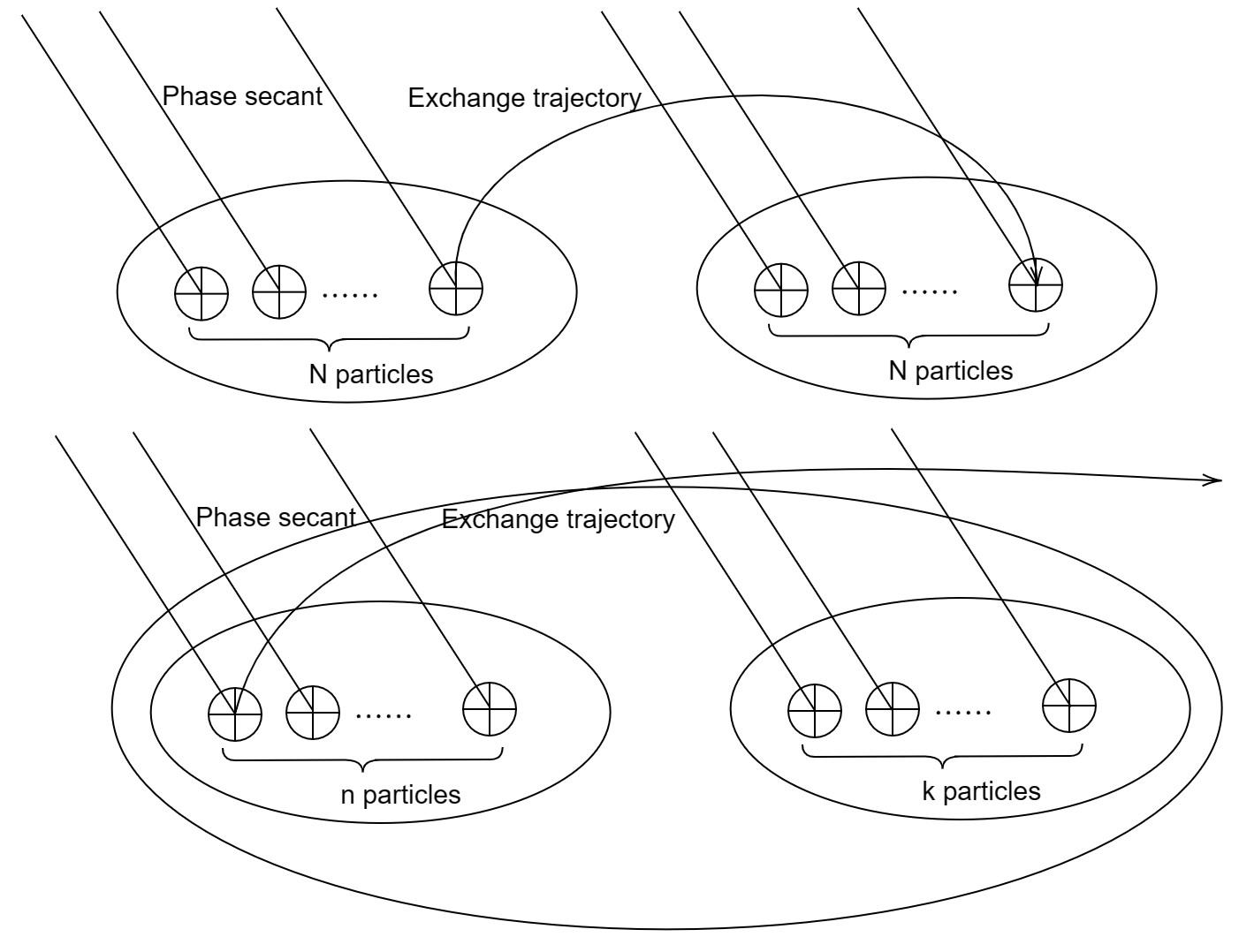
However, in an anyon system, New particles can emerge through fusion, which combines two anyons to form a new quasiparticle. Take Abelian anyons for example. If $\theta_{aa}=\theta$ for type a anyons, then a type b anyon which contains $n$ type a anyons gain $\theta_{bb}=n^2\theta$. Given another type c quasiparticle which contains $k$ particles, a type d particle which is fused by b and c has a statistics $\theta_{dd}=(n+k)^2\theta$. It is shown in 10.
Fusion Law
In the previous section, we have introduced the fusion law for Abelian anyons. Unlike Abelian anyons, non-Abelian anyons may not have a certain fusion channel, which means: \(\phi_a\times\phi_b=\sum_cN_{ab}^c\phi_c\)
The most simple example is SU(2)$_2$ group anyons. This model can be viewed as a spin system that only allows $s\leq 1$ particles (just like our real world). Labelling spin-0 particles as $\mathbf{1}$, spin-$\frac{1}{2}$ particles as $\sigma$, and spin-1 particles as $\psi$. The fusion law is: \(\mathbf{1}\times x= x,x =\mathbf{1},\sigma,\psi\quad \sigma\times\sigma=\mathbf{1}+\psi\quad \psi\times \psi=\mathbf{1}\quad\psi\times\sigma=\sigma\)
An extra channel emerged in $\sigma\times\sigma$.
F matrix
Consider a system with four $\sigma$, labeling 1, 2, 3, and 4 . If we assume all the anyons can fuse to a particle $\mathbf{1}$. Group the particles in pairs, we can expect 1 and 2 fuse to $\mathbf{1}$ (and 3, 4 fuse to $\mathbf{1}$ at the same time) or $\psi$ (and 3, 4 fuse to $\psi$ at the same time). Then the system has a two-dimensional degenerated Hilbert space with basis $\psi_{\mathbf{1}},\psi_\psi$. However, we can also group particles 1, 3 and 2, 4, making a new basis of this Hilbert space $\Tilde{\psi}{\mathbf{1}}$ and $\Tilde{\psi}\psi$.
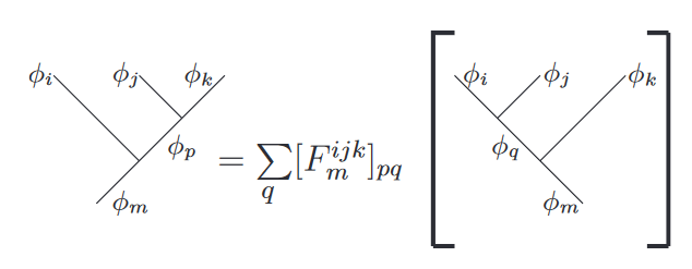
Since both sets of basis are complete, there exists a unitary transformation between them. This is called the $F$ matrix (for fusion). In this specific case, the transformation is: \(\psi_a=F_{ab}\Tilde{\psi}_b\quad a,b=\mathbf{1},\psi\) More generally, the F matrix should be expressed like $F^{ijk}_m$.
R matrix
The different states in this degenerate multianyon state space transform into each other under braiding. However, two particles cannot change their fusion channel simply by braiding with each other, since their total topological charge can be measured along a far distant loop enclosing the two particles. They must braid with a third particle in order to change their fusion channel. Consequently, when two particles fuse in a particular channel rather than a linear superposition of channels, the effect of taking one particle around the other is multiplication by a phase. This phase resulting from a counterclockwise exchange of particles of types a and b which fuse to a particle of type c is called $R^{ab}c$.In the Ising anyon case, as derived in Sec. III and the Appendix, $R_1^{\sigma\sigma} = e^{-\pi i/8}, R\psi^{\sigma\sigma}= e^{3\pi i/8}, R_1^{\psi\psi}=-1, R_\sigma^{\sigma\psi}= i$. For an example of how this works, suppose that we create a pair of $\sigma$ quasiparticles out of the vacuum. They will necessarily fuse to 1. If we take one around another, the state will change by a phase $e^{-\pi i/8}$. If we take a third $\sigma$ quasiparticle and take it around one, but not both, of the first two, then the first two will now fuse to $\psi$, as shown in Sec. III. If we now take one of the first two around the other, the state will change by a phase $e^{3\pi i/8}$.
Physcial Emergence
Fermions and bosons in 2-dimensional material still obey Fermi or Bose statistics, as there are no real 2-dimensional fermion or boson. However, if a system of many electrons or bosons, atoms, etc. confined to a two-dimensional plane has excitations which are localized disturbances of its quantum mechanical ground state, known as quasiparticles, then these quasiparticles can be anyons. When a system has anyonic quasiparticle excitations above its ground state, it is in a topological phase of matter.
BCS Theory
Cooper pair
Define the Cooper pair creation operator as: \(\Lambda^\dagger=\sum_\mathbf{k}\phi_\mathbf{k}c_\mathbf{k}^\dagger c_{-\mathbf{k}\uparrow}^\dagger\quad \phi_\mathbf{k}=\int d^3xe^{-i\mathbf{k}\cdot\mathbf{x}}\phi(\mathbf{x})\) Consider the excitation of a Cooper pair in a system, the added Cooper pair should be in the valance state above the Fermi surface $\ket{FS}$: \(|\Psi\rangle=\Lambda^\dagger|FS\rangle=\sum_{|\mathbf{k}|>k_F}\phi_\mathbf{k}|\mathbf{k}_P\rangle,\) Suppose the system is governed by $H=\sum_\mathbf{k}\epsilon_\mathbf{k}c_\mathbf{k\sigma}^\dagger c_\mathbf{k\sigma}+\hat{V}$, the Schrodinger equation gives: \(\begin{align} H\ket{\Psi}&=E\ket{\Psi}\\ \sum_{|\mathbf{k}|>k_F}2\epsilon_\mathbf{k}\phi_\mathbf{k}|\mathbf{k}_P\rangle+\sum_{|\mathbf{k}|,|\mathbf{k}^{\prime}|>k_F}|\mathbf{k}_P\rangle\langle\mathbf{k}_P|\hat{V}|\mathbf{k}_P^{\prime}\rangle\phi_{\mathbf{k}^{\prime}}&=E\sum_\mathbf{k}\phi_\mathbf{k}|\mathbf{k}_P\rangle \end{align}\) Multiply $\bra{\mathbf k_p}$ in the left: \(E\phi_\mathbf{k}=2\epsilon_\mathbf{k}\phi_\mathbf{k}+\sum_{|\mathbf{k}^{\prime}|>k_F}\langle\mathbf{k}_P|\hat{V}|\mathbf{k}_P^{\prime}\rangle\phi_{\mathbf{k}^{\prime}}\) In a simple approximation, the potential mediated by electron-phonon interaction is a constant attractive potential within a small range $\omega_D$: \(\left.V_{\mathbf{k},\mathbf{k}^{\prime}}=\left\{\begin{array}{ccc}-g_0/V&&(|\epsilon_{\mathbf{k}}|,|\epsilon_{\mathbf{k}^{\prime}}|<\omega_D)\\0&&(\mathrm{otherwise}).\end{array}\right.\right. \label{eq:swaveV}\) Put it back and calculate: \(\begin{align} \phi_\mathbf{k}&=-\frac{g_0/V}{E-2\epsilon_\mathbf{k}}\sum_{0<\epsilon_{\mathbf{k}^{\prime}}<\omega_D}\phi_{\mathbf{k}^{\prime}}\\ \sum_{\mathbf{k}}\phi_\mathbf{k}&=\sum_{0<\epsilon_{\mathbf{k}^{\prime}}<\omega_D}\phi_{\mathbf{k}^{\prime}}\sum_{\mathbf{k}}-\frac{g_0/V}{E-2\epsilon_\mathbf{k}}\\ 1&=-\frac{1}{V}\sum_{0<\epsilon_{\mathbf{k}}<\omega_D}\frac{g_0}{E-2\epsilon_{\mathbf{k}}}\\ 1&=g_0N(0)\int_0^{\omega_D}\frac{d\epsilon}{2\epsilon-E}=-\frac{1}{2}g_0N(0)\ln\left[\frac{2\omega_D-E}{-E}\right]\approx-\frac{1}{2}g_0N(0)\ln\left[\frac{2\omega_D}{-E}\right] \end{align}\) Thus, the energy of Cooper pair is: \(E=-2\omega_De^{-\frac{2}{g_0N(0)}}\label{eq:CooperEnergy}\) For moving with momentum $p$ Cooper pair, the creation operator is: \(\Lambda^\dagger(\mathbf{p})=\sum_\mathbf{k}\phi(\mathbf{k})c_{\mathbf{k}+\mathbf{p}/2\uparrow}^\dagger c_{-\mathbf{k}+\mathbf{p}/2\downarrow}^\dagger\) The further calculation shows: \(E_\mathbf{p}=-2\omega_D\exp\left[-\frac{2}{g_0N(0)}\right]+\mathrm{v}_Fp\) Linear dispersion is associated with the superfluidity/superconductivity.
::: corollary Corollary 1. Superfluid
For the phase field in complex scalar field spontaneous U(1) symmetry breaking: \(\frac{1}{2g^2}\partial_0^2\theta-\frac{\bar\rho}{m}\partial_i^2\theta=0\) In phase space, the solution is a gapless mode: \(\omega^2=\frac{2g^2\bar\rho}{m}\vec k^2\) Linearly dispersing mode implies superfluidity. Considering a bunch of bosons flowing down a tube with mass $M$ and velocity $v$. Its momentum can be decreased by excitation of collective modes, which is actually the mode we derived above. If the mode has a momentum $k$, it should obey: \(\begin{align} Mv=Mv'+\hbar k\\ \frac{1}{2}Mv^2\ge\frac{1}{2}Mv'^2+\hbar\omega(k)\\ \therefore -{\hbar k}v+\frac{1}{2M}\hbar^2k^2+\hbar\omega(k)\le0 \end{align}\) In the macroscopic limit $M\to\infty$, we can obtain $v\ge\frac{\omega}{k}=g\sqrt{\frac{2\bar\rho}{m}}$. This means if the flow velocity is bounded below the critical speed, the flow is super. Scaling the distance ($\partial_i$), we can re write the lagrangian as: \(\mathcal{L}=\frac{1}{4g^2}(\partial_\mu\theta)^2\) This is scale particle like field of phase angle, which represents the spontaneous breaking of the global $\mathrm U(1)$ symmetry.
Considering the example of boson gas, the bosons cannot be independently excited to momontum $k$ because of the repulsion interatction. In $D$ dimensional space, state density $N(E)\propto k^{D-1}(\mathrm d k/\mathrm d E)$.
From Goldstones’ theory, which states that whenever a continuous symmetry is spontaneously broken, massless fields, known as Nambu-Goldstone bosons, emerge. In this example, the bosons is the $\theta$ field. :::
BCS state, order parameter, and Hamiltonian
The superconducting ground state is chosen as the coherent state of the Cooper pair creation operator: \(|\psi_{BCS}\rangle=\prod_{\mathbf{k}}\exp[\phi_{\mathbf{k}}c_{\mathbf{k}\uparrow}^\dagger c_{-\mathbf{k}\downarrow}^\dagger]|0\rangle=\prod_{\mathbf{k}}(1+\phi_{\mathbf{k}}c_{\mathbf{k}\uparrow}^\dagger c_{-\mathbf{k}\downarrow}^\dagger)|0\rangle\) Here have used the property of Fermi statistics $(c_{\mathbf{k}\uparrow}^\dagger c_{-\mathbf{k}\downarrow}^\dagger)^n=0\left(n>1\right)$. The next step is to build Hamiltonian. Besides the kinetic term, the general form of 2-body interaction term should be: \(\langle\hat{V}\rangle=\frac{1}{2}\sum_{ijmn}V_{ijmn}\langle a_i^\dagger a_j^\dagger a_ma_n\rangle\quad V_{ijmn}=\Omega^{-2}\int dr\int dr^{\prime}V(\boldsymbol{r-r}^{\prime})e^{i(\boldsymbol{k_i-k_n})\cdot\boldsymbol{r}}e^{i(\boldsymbol{k_j-k_m})\cdot\boldsymbol{r}^{\prime}}\) There are three possible non-zero cases:
$i=n,j=m$, Hartree Term, a constant $\braket{V}=\frac{1}{2}V(0)N^2$. Ignored.
$i=m,j=n$, Fork Term,
\(H=\sum_{\mathbf{k}\sigma}\epsilon_{\mathbf{k}\sigma}c_{\mathbf{k}\sigma}^\dagger c_{\mathbf{k}\sigma}+\sum_{\mathbf{k},\mathbf{k}^{\prime}}V_{\mathbf{k},\mathbf{k}^{\prime}}c_{\mathbf{k}\uparrow}^\dagger c_{-\mathbf{k}\downarrow}^\dagger c_{-\mathbf{k}^{\prime}\downarrow}c_{\mathbf{k}^{\prime}\uparrow}\) For s-wave manifestation the potential is the Eq. ((eq:swaveV)), then it takes the form: \(\begin{aligned}&H=\sum_{|\epsilon_{\mathbf{k}}|<\omega_{D},\sigma}\epsilon_{\mathbf{k}}c_{\mathbf{k}\sigma}^{\dagger}c_{\mathbf{k}\sigma}-\frac{g_{0}}{\mathrm{V}}A^{\dagger}A.\\&A^{\dagger}=\sum_{|\epsilon_{\mathbf{k}}|<\omega_{D}}c_{\mathbf{k}\uparrow}^{\dagger}c_{-\mathbf{k}\downarrow}^{\dagger},\quad A=\sum_{|\epsilon_{\mathbf{k}^{\prime}}|<\omega_{D}}c_{-\mathbf{k}^{\prime}\downarrow}c_{\mathbf{k}^{\prime}\uparrow}\end{aligned}\) The Order Parameter is set as the density of pair operator: \(\Delta=|\Delta|e^{i\phi}=-\frac{g_0}{\mathrm{V}}\langle\hat{A}\rangle=-g_0\int_{|\epsilon_\mathbf{k}|<\omega_D}\frac{d^3k}{(2\pi)^3}\langle c_{-\mathbf{k}\downarrow}c_{\mathbf{k}\uparrow}\rangle\) The distribution function $\mathcal{P}$ can be expanded because of $\delta S[\delta\Delta]=S[\Delta+\delta\Delta_0]-S[\Delta]\sim \mathrm{V}\times\delta\Delta^2$: \(\mathcal{P}[\Delta]\propto e^{-S[\delta\Delta]}\sim\exp\left[-\frac{\delta\Delta^2}{O(1/\mathrm{V})}\right]\) This supports the mean-field treatment. Using the relation $\delta\hat{A}=\hat{A}-\braket{\hat{A}}=\hat{A}+\frac{\mathrm{V}}{g_0}\Delta$: \(-\frac{g_0}{V}A^\dagger A=\overbrace{\bar{\Delta}A+A^\dagger\Delta+\mathrm V\frac{\bar{\Delta}\Delta}{g_0}}^{O(V)}-\overbrace{\frac{g_0}{\mathrm V}\delta A^\dagger\delta A}^{O(1)}\) In thermodynamic limit, the last term can be neglected. The mean-field BCS Hamiltionian with the order parameter is: \(H_{MFT}=\sum_{\mathbf{k}\sigma}\epsilon_{\mathbf{k}}c_{\mathbf{k}\sigma}^\dagger c_{\mathbf{k}\sigma}+\sum_{\mathbf{k}}\left[\bar{\Delta}c_{-\mathbf{k}\downarrow}c_{\mathbf{k}\uparrow}+c_{\mathbf{k}\uparrow}^\dagger c_{-\mathbf{k}\downarrow}^\dagger\Delta\right]+\frac{V}{g_0}\bar{\Delta}\Delta\) Now focusing on the Pairing term in the MFT Hamiltonian: \(H_P(\mathbf{k})=\left(\bar{\Delta}c_{-\mathbf{k}\downarrow}c_{\mathbf{k}\uparrow}+c_{\mathbf{k}\uparrow}^\dagger c_{-\mathbf{k}\downarrow}^\dagger\Delta\right)\) The term $\bar\Delta c_{-\mathbf k\downarrow}c_{\mathbf{k}\uparrow}$ indicates the annihilation of two electrons and the formation of a Cooper pair. The hole, as the inverse of electron, is created by operator $h^\dagger_{\mathbf{k}\uparrow}=c_{-\mathbf{k}\downarrow}$. Then the pairing term becomes $h^\dagger_{\mathbf{k}\uparrow}\bar\Delta c_{\mathbf{k}\uparrow}+h.c.$. It picture the process $e^-=\mathrm{pair}^{2-}+h^+$, which is called Andreev reflection. Noted:
Andreev reflection reverse all components of the velocity, result in non-specular.
Andreev reflection conserve the spin, momentum and current.
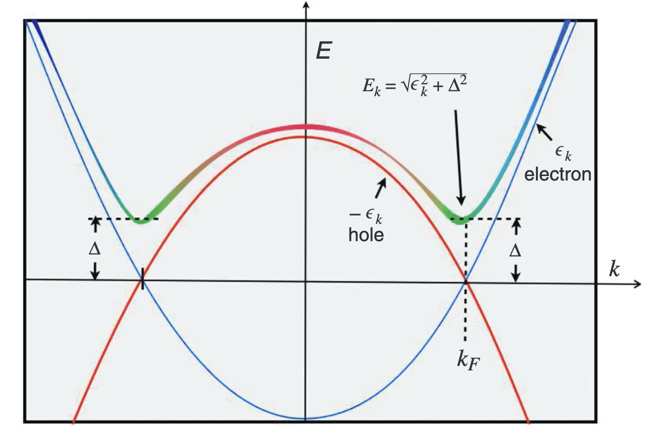
In the band spectrum, the dispersion relation of hole is $-\varepsilon_{-\mathbf{k}}$ as to the dispersion relation of electron $\varepsilon_{\mathbf{k}}$. [($\clubsuit$ TODO: The inversion is not clear. Why set Fermi energy as Zero? $\clubsuit$)]{style=”color: OliveGreen”} Near Fermi surface, the quasiparticle is the mixture of electrons and holes, leading to a gap openning.
Nambu Formalism
Nambu spinor is defined as: \(\psi_{\mathbf{k}}=\begin{pmatrix}c_{\mathbf{k}\uparrow}\\c_{-\mathbf{k}.\downarrow}^\dagger\end{pmatrix}, \psi_{\mathbf{k}}^\dagger=\left(c_{\mathbf{k}\uparrow}^\dagger,c_{-\mathbf{k}\downarrow}\right)\) The anti-commutation relation of Nambu spinor is: \(\begin{align} \{\psi_{\mathbf{k}\alpha},\psi_{\mathbf{k}^{\prime}\beta}^\dagger\}&=\begin{pmatrix} c_{\mathbf{k}\alpha}c^\dagger_{\mathbf{k'}\beta}&c_{\mathbf{k}\alpha}c_{-\mathbf{k'}\beta}\\ c^\dagger_{-\mathbf{k}\beta}c^\dagger_{\mathbf{k'}\alpha}&c^\dagger_{-\mathbf{k}\beta}c_{-\mathbf{k'}\beta} \end{pmatrix}+c^\dagger_{\mathbf{k}\alpha}c_{\mathbf{k'}\alpha}+c_{-\mathbf{k}\beta}c^\dagger_{-\mathbf{k'}\beta}\\ &=\delta_{\alpha\beta}\delta_{\mathbf{k},\mathbf{k'}} \end{align}\) [($\clubsuit$ TODO: The commutation relation is not deduced completely. $\clubsuit$)]{style=”color: OliveGreen”}
The kinetic term of $H_{MFT}$ can be rewritten: \(\begin{align} \sum_{\mathbf{k}\sigma}\epsilon_{\mathbf{k}}c_{\mathbf{k}\sigma}^\dagger c_{\mathbf{k}\sigma}&=\sum_{\mathbf{k}}\epsilon_{\mathbf{k}}(c_{\mathbf{k}\uparrow}^\dagger c_{\mathbf{k}\uparrow}-c_{-\mathbf{k}\downarrow}c_{-\mathbf{k}\downarrow}^\dagger+c_{\mathbf{k}\downarrow}^\dagger c_{\mathbf{k}\downarrow}+c_{-\mathbf{k}\downarrow}c_{-\mathbf{k}\downarrow}^\dagger)\\ &=\sum_{\mathbf{k}}\epsilon_\mathbf{k}(c_{\mathbf{k}\uparrow}^\dagger c_{\mathbf{k}\uparrow}-c_{-\mathbf{k}\downarrow}c_{-\mathbf{k}\downarrow}^\dagger+1)\\&=\begin{pmatrix}c_{\mathbf{k}\uparrow}^\dagger,c_{-\mathbf{k}\downarrow}\end{pmatrix}\begin{bmatrix}\epsilon_\mathbf{k}&0\\0&-\epsilon_\mathbf{k}\end{bmatrix}\begin{pmatrix}c_{\mathbf{k}\uparrow}\\\bar{c}_{-\mathbf{k}\downarrow}^\dagger\end{pmatrix}+\sum_\mathbf{k}\epsilon_\mathbf{k} \end{align}\) [($\clubsuit$ TODO: Why here is valid??? $\clubsuit$)]{style=”color: OliveGreen”}
Drop the constant term, the hole Hamiltonian can be rewritten: \(\begin{align}\epsilon_{\mathbf{k}}\sum_\sigma c_{\mathbf{k}\sigma}^\dagger c_{\mathbf{k}\sigma}+\left[\bar{\Delta}c_{-\mathbf{k}\downarrow}c_{\mathbf{k}\uparrow}+c_{\mathbf{k}\uparrow}^\dagger c_{-\mathbf{k}\downarrow}^\dagger\Delta\right]&=\begin{pmatrix}c_{\mathbf{k}\uparrow}^\dagger,c_{-\mathbf{k}\downarrow}\end{pmatrix}\begin{bmatrix}\epsilon_\mathbf{k}&\Delta\\\bar{\Delta}&-\epsilon_\mathbf{k}\end{bmatrix}\begin{pmatrix}c_{\mathbf{k}\uparrow}\\c_{-\mathbf{k}\downarrow}^\dagger\end{pmatrix}\\&=\psi_\mathbf{k}^\dagger\begin{bmatrix}\epsilon_\mathbf{k}&\Delta_1-i\Delta_2\\\Delta_1+i\Delta_2&-\epsilon_\mathbf{k}\end{bmatrix}\psi_\mathbf{k}\\&=\psi_k^\dagger[\epsilon_k\tau_3+\Delta_1\tau_1+\Delta_2\tau_2]\psi_k,\end{align} \label{eq:Nambu}\) here use the isospin matrix: \(\vec{\tau}=(\tau_1,\tau_2,\tau_3)=\left(\begin{bmatrix}0&1\\1&0\end{bmatrix},\begin{bmatrix}0&-i\\i&0\end{bmatrix},\begin{bmatrix}1&0\\0&-1\end{bmatrix}\right)\) Putting this all together: \(H=\sum_\mathbf{k}\psi_\mathbf{k}^\dagger(\vec{h}_\mathbf{k}\cdot\vec{\tau})\psi_\mathbf{k}+V\frac{\bar{\Delta}\Delta}{g_0}\quad \vec{h}_\mathbf{k}=(\Delta_1,\Delta_2,\epsilon_\mathbf{k})\)
Discrete Formalism
The derivation here is following the Senthil’s work[@senthil_spin_1999]. Denote $i,j$ as the index of sites, the discrete form of MFT hamiltonian is: \(\mathcal{H}=\sum_{i,j}\left[t_{ij}\sum_\alpha c_{i\alpha}^\dagger c_{j\alpha}+\Delta_{ij}c_{i\uparrow}^\dagger c_{\downarrow j}^\dagger+\Delta_{ij}^*c_{j\downarrow}c_{i\uparrow}\right]\) $t_{ij}=t_{ij}^*$ due to hermiticity, $\Delta_{ij}=\Delta_{ji}$ due to spin rotation invariance (Hamiltonian should be invariant when choosing particle $i$ spin down and $j$ spin up. The discrete Nambu formalism is: \(\begin{align} \psi_i = \begin{pmatrix} c_{i\uparrow}\\c_{i\downarrow}^\dagger \end{pmatrix} \end{align}\)
Anderson’s domain-wall
The isospin operator is defined as: \(\vec \tau_{\mathbf{k}}=\psi_{\mathbf{k}}^\dagger\vec\tau\psi_{\mathbf{k}}\) which means: \(\begin{align} \tau_{3\mathbf{k}}&=\psi_\mathbf{k}^\dagger\tau_3\psi_\mathbf{k}=(c_{\mathbf{k}\uparrow}^\dagger c_{\mathbf{k}\uparrow}-c_{-\mathbf{k}\downarrow}c_{-\mathbf{k}\downarrow}^\dagger)=(n_{\mathbf{k}\uparrow}+n_{-\mathbf{k}\downarrow}-1)\\ \hat{\tau}_{1\mathbf{k}}&=\psi_{\mathbf{k}}^\dagger\tau_1\psi_{\mathbf{k}}=\quad c_{\mathbf{k}\uparrow}^\dagger c_{-\mathbf{k}\downarrow}^\dagger+c_{-\mathbf{k}\downarrow}c_{\mathbf{k}\uparrow}\\ \hat{\tau}_{2\mathbf{k}}&=\psi_{\mathbf{k}}^\dagger\tau_2\psi_{\mathbf{k}}=-i(c_{\mathbf{k}\uparrow}^\dagger c_{-\mathbf{k}\downarrow}^\dagger-c_{-\mathbf{k}\downarrow}c_{\mathbf{k}\uparrow})\\ \tau_{+\mathbf{k}}&=\tau_{1\mathbf{k}}+i\tau_{2\mathbf{k}}=2c_{\mathbf{k}\uparrow}^\dagger c_{-\mathbf{k}\downarrow}^\dagger\\ \tau_{-\mathbf{k}}&=\tau_{1\mathbf{k}}-i\tau_{2\mathbf{k}}=-2c_{\mathbf{k}\uparrow} c_{-\mathbf{k}\downarrow} \end{align}\) Note that: \(=-2\tau_{+\mathbf{k}}\quad[\tau_{+\mathbf{k}},\tau_{-\mathbf{k}}]=4(n_{\mathbf{k\uparrow}}+n_{\mathbf{-k\downarrow}}-1)=4\tau_{3\mathbf{k}}\) This shows the isospin operators form $\mathfrak{su}(2)$ Lie algebra. Unlike spin operator, the isospin operators are in the charge space. The weights of $\mathfrak{su}(2)$, also the eigenvalue of $\tau_{3\mathbf{k}}$, is $\pm1$, physically meaning the occupation number of Cooper pair state: \(\begin{aligned}&\tau_{3\mathbf{k}}=+1:\quad|\uparrow_{\mathbf{k}}\rangle\quad\equiv\quad|2\rangle=c_{\mathbf{k}\uparrow}^\dagger c_{-\mathbf{k}\downarrow}^\dagger|0\rangle\\&\tau_{3\mathbf{k}}=-1:\quad|\downarrow_{\mathbf{k}}\rangle\quad\equiv\quad|0\rangle.\end{aligned}\) The Hamiltonian of BCS is: \(H_{MFT}=\sum_{\mathbf{k}}\vec\tau_{\mathbf k}\cdot\vec h_{\mathbf{k}}+V\frac{\bar{\Delta}\Delta}{g_0}\) The vector field $\vec B_{\mathbf{k}}=-\vec h_{\mathbf{k}}$ is called Weiss Field. [($\clubsuit$ TODO: Weiss Field is not fully understood, maybe related to Ising model. $\clubsuit$)]{style=”color: OliveGreen”} The Bogoliubov quasiparticle pair is the reversal of an isospin, which cost energy: \(E_\mathbf{k}\equiv|\vec{B}_\mathbf{k}|=\sqrt{\epsilon_\mathbf{k}^2+|\Delta|^2}\) The excitation is gapped in superconductor because of $\Delta\neq0$. In the ground state, each isospin will align parallel to $\vec B_{\mathbf{k}}=-E_{\mathbf{k}}\hat{n_{\mathbf{k}}}, E_{\mathbf{k}}=\sqrt{\epsilon_{\mathbf{k}}^2+|\Delta|^2}$. Mannually setting $\Delta_2=0$: \(\hat{n}_\mathbf{k}=\left(\frac{\Delta_1}{E_\mathbf{k}},\frac{\Delta_2}{E_\mathbf{k}},\frac{\epsilon_\mathbf{k}}{E_\mathbf{k}}\right)=\left(\sin\theta_{\mathbf{k}},0,\cos\theta_{\mathbf{k}}\right)\) In normal metal, $\langle\tau_{3\mathbf{k}}\rangle=\langle n_{\mathbf{k}\uparrow}+n_{-\mathbf{k}\downarrow}-1\rangle=\mathrm{sgn}(k_F-k)$. However, in the superconductor: \(\langle\tau_{3\mathbf{k}}\rangle=\langle n_{\mathbf{k}\uparrow}+n_{-\mathbf{k}\downarrow}-1\rangle=-\cos\theta_{\mathbf{k}}=-\frac{\epsilon_{\mathbf{k}}}{\sqrt{\epsilon_{\mathbf{k}}^2+\Delta^2}}\) Align the two equations: \(\begin{align} \langle\tau_{1\mathbf{k}}\rangle&=\langle(c_{\mathbf{k}\uparrow}^\dagger c_{-\mathbf{k}\downarrow}^\dagger+c_{-\mathbf{k}\downarrow}c_{\mathbf{k}\uparrow})\rangle=-\sin\theta_\mathbf{k}=-\frac{\Delta}{\sqrt{\epsilon_\mathbf{k}^2+\Delta^2}}\\ \langle\tau_{2\mathbf{k}}\rangle&=-i\langle(c_{\mathbf{k}\uparrow}^\dagger c_{-\mathbf{k}\downarrow}^\dagger-c_{-\mathbf{k}\downarrow}c_{\mathbf{k}\uparrow})\rangle=0 \end{align}\) We can get the gap function in zero temperature: \(\Delta=-\frac{g_0}{\mathrm{V}}\sum_{\mathbf{k}}\braket{c_{-\mathbf{k}\downarrow}c_{\mathbf{k}\uparrow}}=\frac{g_0}{\mathrm V}\sum_\mathbf{k}\frac{1}{2}\sin\theta_\mathbf{k}=g_0\int_{|\epsilon_\mathbf{k}|<\omega_D}\frac{d^3k}{(2\pi)^3}\frac{\Delta}{2\sqrt{\epsilon_\mathbf{k}^2+\Delta^2}}\) In approximation: \(\Delta=2\omega_De^{-\frac{1}{g_0N(0)}}\)
The symmetry of pairing
A more generalized form of superconducting Hamiltonian, allowing the spin triplet scenario: \(\begin{aligned}H&=\quad H_0+H_{int}\\&=\quad\sum_{\boldsymbol{k}ss^{\prime}}H_0(\boldsymbol{k})c_{\boldsymbol{k}s}^\dagger c_{\boldsymbol{k}s^{\prime}}+\frac{1}{2}\sum_{\boldsymbol{k}\boldsymbol{k}^{\prime}s_1s_2s_3s_4}V_{\boldsymbol{s}_1s_2s_3s_4}(\boldsymbol{k},\boldsymbol{k}^{\prime})c_{\boldsymbol{k}s_1}^\dagger c_{-\boldsymbol{k}s_2}^\dagger C_{\boldsymbol{k}^{\prime}s_3}C_{-\boldsymbol{k}^{\prime}s_4}\end{aligned}\) The generalized form of pair function is: \(\Delta_{s_1s_2}(\boldsymbol{k})\quad=\quad\frac{1}{\boldsymbol{N}}\sum_{\boldsymbol{k}^{\prime}s_3s_4}V_{s_1s_2s_3s_4}(\boldsymbol{k},\boldsymbol{k}^{\prime})\langle c_{\boldsymbol{k}^{\prime}s_3}c_{-\boldsymbol{k}^{\prime}s_4}\rangle,\) With the generalized Nambu basis: \(\Psi_{\mathbf{k}}=\left(c_{\mathbf{k}\uparrow},c_{\mathbf{k}\downarrow},c_{-\mathbf{k}\uparrow}^{\dagger},c_{-\mathbf{k}\downarrow}^{\dagger}\right)^{T},\) The matrix rep. of superconducting Hamiltonian has the similar form to Eq. ((eq:Nambu)), with 4 dimension, called BdG Hamiltonian: \(H_{BdG}(\boldsymbol{k})=\begin{bmatrix}H_0(\boldsymbol{k})&\Delta(\boldsymbol{k})\\\\\Delta^\dagger(\boldsymbol{k})&-H_0^t(\boldsymbol{-k})\end{bmatrix}\) Because a Cooper pair is made of identical fermions, its two–particle wavefunction must be antisymmetric under exchanging the two electrons. This means a minus sign emerges under exchanges below: \((\mathbf{k},s_1)\longleftrightarrow(-\mathbf{k},s_2),\) So, \(\begin{align} \Delta_{s_2 s_1}(-\mathbf{k})&=\quad\frac{1}{\boldsymbol{N}}\sum_{\boldsymbol{k}^{\prime}s_3s_4}V_{s_2s_1s_3s_4}(\boldsymbol{-k},\boldsymbol{k}^{\prime})\langle c_{\boldsymbol{k}^{\prime}s_3}c_{\boldsymbol{-k}^{\prime}s_4}\rangle\\ &=\quad\frac{1}{\boldsymbol{N}}\sum_{\boldsymbol{k}^{\prime}s_3s_4}-V_{s_1s_2s_3s_4}(\boldsymbol{k},\boldsymbol{k}^{\prime})\langle c_{\boldsymbol{k}^{\prime}s_3}c_{\boldsymbol{-k}^{\prime}s_4}\rangle\\ &=-\Delta_{s_1s_2}(\mathbf{k}) \Delta(\mathbf{k}) = -\Delta(\mathbf{-k})^T \end{align}\) This is based on the properties of interactional matrix: \(\begin{align} V_{s_1s_2s_3s_4}(\boldsymbol{k},\boldsymbol{k}^{\prime})=\bra{s_1,\mathbf{k};s_2,\mathbf{-k}}V\ket{s_3,\mathbf{k'};s_4,\mathbf{-k'}}\\ V_{s_2s_1s_3s_4}(\boldsymbol{-k},\boldsymbol{k}^{\prime})=\bra{s_2,\mathbf{-k};s_1,\mathbf{k}}V\ket{s_3,\mathbf{k'};s_4,\mathbf{-k'}}=-V_{s_1s_2s_3s_4}(\boldsymbol{k},\boldsymbol{k}^{\prime}) \end{align}\) Due to the constrain on the matrix, the matrix rep. of spin singlet is chosen to be $\phi(\mathbf k) i\sigma_y$ ($(i\sigma_y)^T=-i\sigma_y$), the following matrix reps. of spin triplet are denoted to be $i \mathbf{d}(\mathbf{k})\cdot\mathbf{\sigma}\sigma_y$, composing a complete basis of SU(2). $\phi$ and $d_i$ are the C-G coefficients.
Cuprates
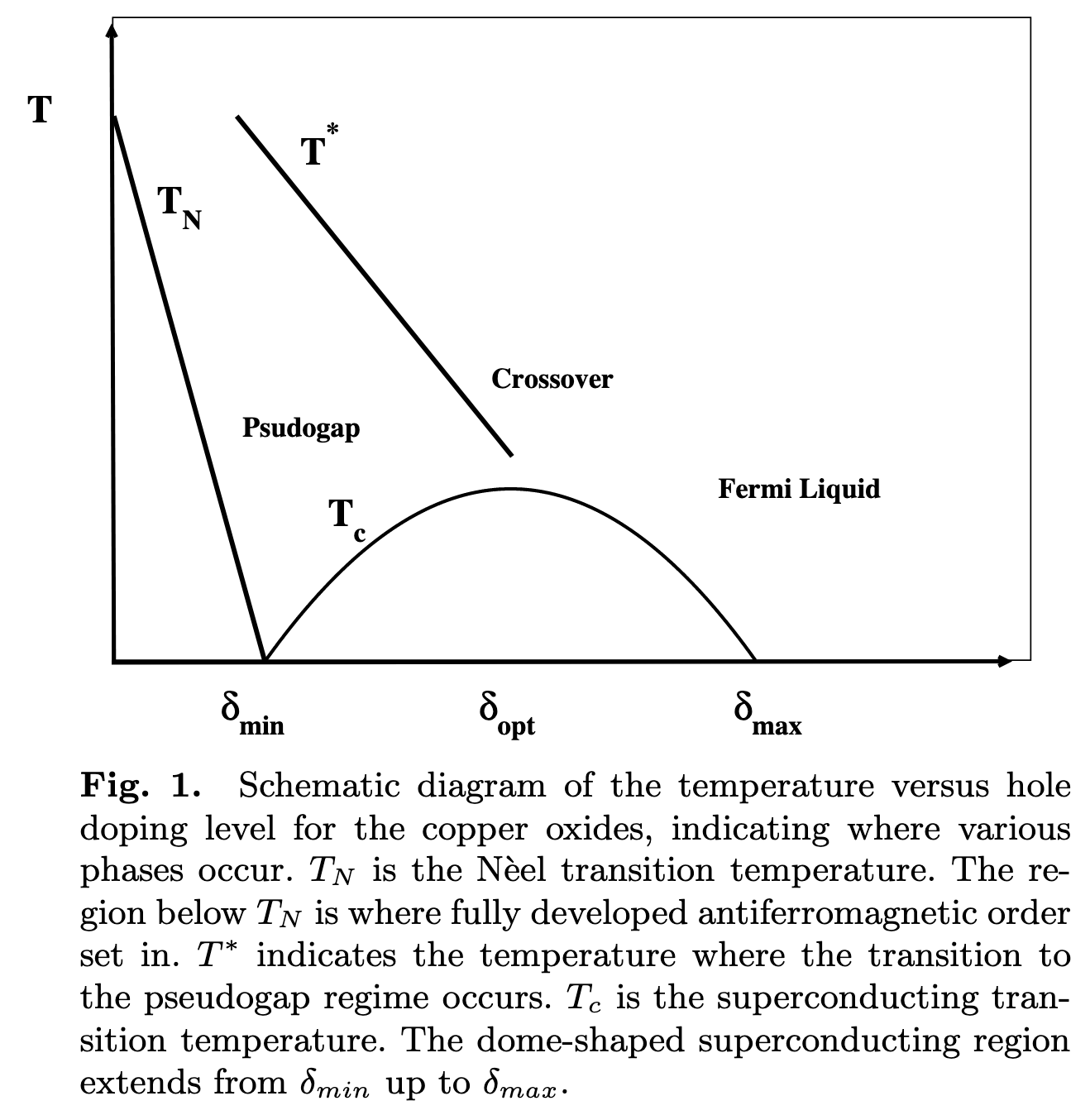
The superconductivity of cuprates is related to the square planar CuO$_2$. Effective Habbard Model can describe: \(\hat{H}=-t\sum_{<i,j>,\sigma}\left[\hat{c}_{i,\sigma}^\dagger\hat{c}_{j,\sigma}+\hat{c}_{j,\sigma}^\dagger\hat{c}_{i,\sigma}\right]+U\sum_i\hat{n}_{i,\uparrow}\hat{n}_{i,\downarrow},\hat{n}_{i,\sigma}=\hat{c}_{i,\sigma}^\dagger\hat{c}_{i,\sigma}.\) $U$ is on-site Coulomb repulsion between opposite spin electrons on the same site. The first term considering the spin coupling between nearest neighbours $i,j$, yielding the Heisenberg antiferromagnetic exchange interaction with $J = \frac{4t^2}{U}$.
Simplified Assumption:
CuO$_2$ contributes to the superconductivity.
One band superconductivity.
In Habbard Model, there can have 0, 1, or 2 electrons at each site. When $U\gg t$, the double-occupied states have sufficient high energy. When we consider the propagation of holes, it is analogy to the inverse hopping of electrons. However, if electrons hopping to the single-occupied sites, the system raise energy due to the new double-occupied state. In a low energy approximation, we focus on the low energy subspace, which means the electron occupation number $\leq 1$.
The complete space of the electrons in cuprate can be divided into the low energy space $S_0$ and the high energy space $S_1$, where the projection operators are $P$ and $Q$ seperately.
Block decomposition of an operator with respect to subspaces {#block-decomposition-of-an-operator-with-respect-to-subspaces .unnumbered}
Let the Hilbert space decompose into a direct sum $\mathcal H=\mathrm{Im}\,P\oplus\mathrm{Im}\,Q=:\mathcal H_P\oplus\mathcal H_Q$, where the orthogonal projectors satisfy \(\begin{aligned} P^2=P,\quad Q^2=Q,\quad PQ=QP=0,\quad P+Q=\mathbb 1. \end{aligned}\) For any linear operator $H:\mathcal H\to\mathcal H$, inserting the identity into both sides gives \(\begin{aligned} H=(P+Q)H(P+Q)=PHP+PHQ+QHP+QHQ. \label{eq:block-expansion} \end{aligned}\) Take an arbitrary vector $v\in\mathcal H$ and split it as $v=x+y$ with $x=Pv\in\mathcal H_P,\ y=Qv\in\mathcal H_Q$. Then, from (eq:block-expansion), \(\begin{aligned} Hv&=(PHP+PHQ+QHP+QHQ)(x+y)\\ &=(PHP\,x+PHQ\,y)+(QHP\,x+QHQ\,y). \end{aligned}\) Thus the components of $Hv$ in each subspace are \(\begin{aligned} PHv=PHP\,x+PHQ\,y,\qquad QHv=QHP\,x+QHQ\,y. \label{eq:components} \end{aligned}\) Representing the vector and its image by column vectors of their components, $v\widehat{=}\binom{x}{y},\ Hv\widehat{=}\binom{PHv}{QHv},$ equation (eq:components) yields \(\begin{aligned} Hv\ \widehat{=}\ \begin{pmatrix} PHP & PHQ\\ QHP & QHQ \end{pmatrix} \binom{x}{y}. \end{aligned}\) Therefore, in a basis adapted to the direct sum $\mathcal H=\mathcal H_P\oplus\mathcal H_Q$, the operator $H$ admits the block representation \(\begin{aligned} H\ \widehat{=}\ \begin{pmatrix} PHP & PHQ\\ QHP & QHQ \end{pmatrix}. \end{aligned}\) In this form, each block has a clear meaning: $PHP:\mathcal H_P\to\mathcal H_P$, $PHQ:\mathcal H_Q\to\mathcal H_P$, $QHP:\mathcal H_P\to\mathcal H_Q$, and $QHQ:\mathcal H_Q\to\mathcal H_Q$.
From Hubbard to the projected $t$–$J$+$!$three-site effective Hamiltonian {#from-hubbard-to-the-projected-tjthree-site-effective-hamiltonian .unnumbered}
Setup.
Write the Hubbard Hamiltonian as $H=H_U+H_t$ with \(\begin{aligned} H_U&=U\sum_i n_{i\uparrow}n_{i\downarrow},\\ H_t&=-t\sum_{\langle ij\rangle,s}\!\left(c^\dagger_{is}c_{js}+c^\dagger_{js}c_{is}\right). \end{aligned}\) Let $P$ project onto the no-double-occupancy subspace $\mathcal S_0$, and $Q=\mathbb 1-P$ onto its orthogonal complement. To second order in $t/U$ (Schrieffer–Wolff / degenerate perturbation), \(\begin{aligned} H_{\rm eff}=PHP+PHQ\frac{1}{E_0-QHQ}QHP. \end{aligned}\) Since $QHQ=QH_UQ+\mathcal O(t)$ and intermediate states contain exactly one double occupancy, \(\begin{aligned} \frac{1}{E_0-QHQ}=\frac{1}{-QH_UQ}+\mathcal O\!\left(\frac{t}{U^2}\right)\simeq -\frac{1}{U}. \end{aligned}\) Hence, \(\begin{aligned} H_{\rm eff}\simeq PHP-\frac{1}{U}PH_tQH_tP. \label{eq:Heff-second} \end{aligned}\)
(i) Projected nearest-neighbor hopping $H_1$.
The first term gives the projected kinetic energy: \(\begin{aligned} H_1&:=PHP=PH_tP =-t\sum_{\langle ij\rangle,s}\!\left(\tilde c^\dagger_{is}\tilde c_{js}+\text{h.c.}\right),\\ \tilde c_{is}&:=c_{is}\,(1-n_{i\bar s}),\qquad \tilde c^\dagger_{is}:=(1-n_{i\bar s})\,c^\dagger_{is}, \end{aligned}\) which forbids creating double occupancy at either end of the hop.
(ii) Superexchange $H_2$.
In $PH_tQH_tP$ take the process that hops $j!\to! i$ and back $i!\to! j$ on the same bond $\langle ij\rangle$, creating and then removing a virtual double occupancy at energy cost $U$: \(\begin{aligned} H_2&:=-\frac{1}{U}\,P\!\left[-t\!\sum_{\langle ij\rangle,s}c^\dagger_{is}c_{js}\right] \!\left[-t\!\sum_{\langle ij\rangle,s'}c^\dagger_{js'}c_{is'}\right]\!P+\text{h.c.} \end{aligned}\) Using fermion identities and the standard spin representation $\mathbf S_i=\frac{1}{2}\sum_{\alpha\beta}c^\dagger_{i\alpha}\boldsymbol\sigma_{\alpha\beta}c_{i\beta}$ together with \(\begin{aligned} \sum_{ss'}c^\dagger_{is}c_{js}c^\dagger_{js'}c_{is'} = -2\left(\mathbf S_i\!\cdot\!\mathbf S_j-\tfrac{1}{4}n_in_j\right), \end{aligned}\) one obtains the Heisenberg superexchange \(\begin{aligned} H_2=J\sum_{\langle ij\rangle}\!\left(\mathbf S_i\!\cdot\!\mathbf S_j-\tfrac{1}{4}n_in_j\right), \qquad J=\frac{4t^2}{U}. \end{aligned}\)
(iii) Three-site (correlated-hopping) term $H_3$.
The remaining contributions in $PH_tQH_tP$ involve two different bonds sharing the intermediate site $j$ (i.e. $i!-!j$ then $j!-!k$ with $i\neq k$): \(\begin{aligned} H_3&:=-\frac{1}{U}\sum_{\langle ij\rangle,\langle jk\rangle}\! P\left(\sum_s c^\dagger_{is}c_{js}\right) \left(\sum_{s'} c^\dagger_{js'}c_{ks'}\right)P+\text{h.c.} \label{eq:H3-start} \end{aligned}\) After projecting to $\mathcal S_0$ and arranging number operators at $j$, one convenient form is \(\begin{aligned} H_3&=-\frac{t^2}{U}\sum_{\langle ij\rangle,\langle jk\rangle,s}\! \Big( \tilde c^\dagger_{is}\,n_{j\bar s}\,\tilde c_{ks} -\tilde c^\dagger_{i\bar s}\,\tilde c^\dagger_{js}\,\tilde c_{j\bar s}\,\tilde c_{ks} \Big)+\text{h.c.} \label{eq:H3-operator} \end{aligned}\) It describes correlated hopping from $i$ to $k$ through $j$ conditioned on the spin/occupancy at $j$. In an antiferromagnetic background (and dilute-hole limit), (eq:H3-operator) reduces effectively to next-nearest-neighbor hole motion on a single sublattice with amplitude $-t^2/U$: \(\begin{aligned} H_3\ \Rightarrow\ -\frac{t^2}{U}\sum_{r}\sum_{i,j}^{\text{NN dirs},\,i\neq -j}\! \psi_h^\dagger(r+i a_0+j a_0)\,\psi_h(r). \end{aligned}\)
Result.
Collecting the pieces, \(\begin{aligned} H_{\rm eff}=H_1+H_2+H_3+\mathcal O\!\left(\frac{t^3}{U^2}\right), \end{aligned}\) where $H_1$ is the projected NN hopping, $H_2$ the superexchange with $J=4t^2/U$, and $H_3$ the three-site (correlated next-nearest) hopping responsible for effective hole propagation on a single sublattice in an AF background.
The physical picture of the hole propagation is that: in half-filling scenario, double occupied states cannot sustain in low-energy situation. So when
From the single–hole effective Hamiltonian to an attractive two–hole potential {#from-the-singlehole-effective-hamiltonian-to-an-attractive-twohole-potential .unnumbered}
Step 1. Single–hole kinetic term.
In the AF background approximation, a hole can only propagate on the same sublattice through a two–step virtual process. The effective kinetic Hamiltonian reads \(\begin{aligned} H_{\rm kin} =-t_{\rm eff}\sum_{r}\sum_{i\neq -j}\sum_{\sigma} \,h^\dagger_{r+i a_0+j a_0,\sigma}\,h_{r,\sigma}, \qquad t_{\rm eff}=\frac{t^2}{U}. \label{eq:Hkin} \end{aligned}\) Here $h_{r,\sigma}$ annihilates a hole with spin $\sigma$ at site $r$, and the restriction $i\neq -j$ ensures that only next–nearest–neighbor hops (same sublattice) appear.
Step 2. Exchange energy in the AF background.
The superexchange term is \(\begin{aligned} H_J =J\sum_{\langle ij\rangle}\Big(\mathbf S_i\!\cdot\!\mathbf S_j-\tfrac{1}{4}n_i n_j\Big), \qquad J=\frac{4t^2}{U}. \end{aligned}\) In the AF background approximation, the spin correlation on an occupied bond is $\langle\mathbf S_i!\cdot!\mathbf S_j\rangle_{\rm AF}=\kappa_{ij}<0$. If either end of the bond is empty (a hole), this correlation vanishes. Thus \(\begin{aligned} H_J^{\rm(AF)} \simeq \sum_{\langle ij\rangle}\Big[J\,\kappa_{ij}-\tfrac{J}{4}\,n_i n_j\Big] =\mathrm{const}-\sum_{\langle ij\rangle}\varepsilon_{ij}\,n_i n_j, \qquad \varepsilon_{ij}=J\Big(\tfrac{1}{4}-\kappa_{ij}\Big)>0. \label{eq:HJ_ninj} \end{aligned}\) Interpretation: AF exchange lowers the energy only if both sites are occupied by electrons. If a hole is present, the bond’s favorable exchange energy is lost.
Step 3. Rewrite in terms of hole number operators.
Define the hole number operator $h_i=\sum_\sigma h^\dagger_{i\sigma}h_{i\sigma}$. In the no–double–occupancy subspace, $n_i=1-h_i$. Then \(\begin{aligned} \sum_{\langle ij\rangle}n_i n_j &=\sum_{\langle ij\rangle}(1-h_i)(1-h_j) =N_{\rm bond}-z\sum_i h_i+\sum_{\langle ij\rangle}h_i h_j. \end{aligned}\) Substituting into (eq:HJ_ninj) and absorbing the constant and linear terms into the chemical potential yields an explicit two–body interaction: \(\begin{aligned} H_{\rm int}^{(2)}=-\sum_{\langle ij\rangle}\varepsilon_{ij}\,h_i h_j, \qquad \varepsilon_{ij}=J\Big(\tfrac{1}{4}-\kappa_{ij}\Big)>0. \label{eq:H2hole_nn} \end{aligned}\) Thus two holes sitting on the ends of a nearest–neighbor bond $\langle ij\rangle$ gain an energy $-\varepsilon_{ij}$. This is precisely an attractive potential between nearest–neighbor holes.
Step 4. Binding–energy estimate.
In a simple “broken–bond” counting argument: - An isolated hole removes $z$ AF bonds. - Two distant holes remove $2z$ bonds in total. - Two adjacent holes share one bond, so they remove only $2z-1$. This reduces the energy relative to the distant case by approximately $\varepsilon_{ij}$.
Numerically, with $\kappa_{ij}=-3/4$ (perfect singlet) one finds $\varepsilon_{ij}=J$. With the actual 2D Heisenberg ground state value $\kappa_{ij}\approx -0.334$, one obtains $\varepsilon_{ij}\approx 0.58\,J$.
Step 5. Extend to finite AF correlation length.
In a system with AF correlation length $\xi_{\rm AF}$, the spin correlation function behaves as \(\begin{aligned} \kappa(\mathbf r)=\langle \mathbf S_0\!\cdot\!\mathbf S_{\mathbf r}\rangle \simeq -\,\kappa_0\,\cos(\mathbf Q\!\cdot\!\mathbf r)\,f(r/\xi_{\rm AF}),\qquad \mathbf Q=(\pi,\pi), \end{aligned}\) with $f(x)\sim K_0(x)$ or $e^{-x}/\sqrt{x}$ in 2D. Substituting into the definition $\varepsilon(\mathbf r)=J(1/4-\kappa(\mathbf r))$ yields a spatially extended two–hole potential \(\begin{aligned} V_{\rm eff}(\mathbf r)\,h_0 h_{\mathbf r},\qquad V_{\rm eff}(\mathbf r)=-\,\varepsilon(\mathbf r) =-\,J\Big(\tfrac{1}{4}-\kappa(\mathbf r)\Big). \label{eq:Veff_r} \end{aligned}\) For distances $a_0\ll r\ll \xi_{\rm AF}$ and sublattice configurations consistent with the Néel pattern, $V_{\rm eff}(\mathbf r)<0$, i.e. attractive. Its magnitude decreases with $r$ according to $f(r/\xi_{\rm AF})$.
Step 6. Effective two–hole Hamiltonian.
Combining the kinetic term (eq:Hkin) with the interaction (eq:H2hole_nn)–(eq:Veff_r), the effective Hamiltonian for two holes reads \(\begin{aligned} H_{\rm pair} &=-t_{\rm eff}\sum_{r}\sum_{i\neq -j}\sum_{\sigma}h^\dagger_{r+i a_0+j a_0,\sigma}\,h_{r,\sigma} +\sum_{\mathbf r}V_{\rm eff}(\mathbf r)\,h_0 h_{\mathbf r} -\mu_h\sum_i h_i+\cdots. \end{aligned}\) The AF background forces the two holes to form a spin singlet. The staggered factor $\cos(\mathbf Q!\cdot!\mathbf r)$ makes the pairing kernel strongest near momentum $(\pi,\pi)$, favoring a $d_{x^2-y^2}$ symmetry.
Summary.
Starting from the single–hole effective Hamiltonian, the AF exchange term, when expressed in terms of hole operators, automatically generates a nearest–neighbor attractive two–body potential. Extending the spin correlation to finite correlation length produces a spatially decaying attractive interaction for $a_0\ll r\ll \xi_{\rm AF}$. Together with the coherent two–step hole hopping, this provides the microscopic basis for the “effective attraction” and possible $d$-wave pairing discussed by Schrieffer, Wen, and Zhang.
Majorana Zero Mode
Intrinsic p-wave superconductor
Using Nambu formalism listed above Eq. ((eq:Nambu)): \(\hat{H}=\begin{bmatrix}\hat{h}&\hat{\Delta}\\\hat{\Delta}^\dagger&-\hat{h}^T\end{bmatrix}\quad \hat{h}=\left(-\frac{1}{2m}\nabla^2-\epsilon_f\right)I\) Contrary to the spherical symmetry function in s-wave pairing Superconductor, the gap function here should be skew symmetry here. The general form of gap function is[@volovikFermionZeroModes1999a]: \(\begin{align} \text{spin singlet:}\quad\Delta=\Delta(\mathbf{r})(\hat{p}_x+i\hat{p}_y)^N\hat{p}_z^{l-|N|},\quad\mathrm{odd~}l,\\\text{spin triplet:}\quad\Delta=\sigma_2\Delta(\mathbf{r})(\hat{p}_x+i\hat{p}_y)^N\hat{p}_z^{l-|N|},\quad\mathrm{even~}l. \end{align}\) For s-wave superconductor, $N=l=0$. For p-wave superconductor, $l=1$. Specifically, $N=l=1$ for $^3$He superfluid. From more recent article[@stone_edge_2004], we set the gap function as: \(\begin{align} \hat{\Delta}=&\frac{1}{2}\left(\frac{\Delta}{k_f}\right)e^{i\Phi/2}\{\hat{\sum},\hat{P}\}e^{i\Phi/2}\\ \Sigma_{\alpha\beta}{=}[i(\boldsymbol{\sigma}{\cdot}\mathbf{d})\sigma_2]_{\alpha\beta}&,\hat{P}=-i(\hat{p}_x+i\hat{p}_y)=-(\partial_x+i\partial_y) \end{align}\) [($\clubsuit$ TODO: The formalism of gap function needs ab-initial derivation. $\clubsuit$)]{style=”color: OliveGreen”} Here $\Phi$ is the overall phase, $\mathbf{d}$ is a unit spin vector. The anti-commutator and the symmetric configuration of $\Phi$ is used for antisymmetric configuration of $\Delta$ when $\Delta(\mathbf{r}),\Sigma,\Phi$ varies in space.
Rectangular geometry
Set the wave function as: \(\Psi=\begin{bmatrix}a\\b\end{bmatrix}e^{ik_xx+ik_yy}\) Apply Fourier transformation to wavefunction and hamiltonian: \(\hat H=\begin{bmatrix} \epsilon(\mathbf{k})&\frac{\Delta}{k_f}(k_x+ik_y)\\ \frac{\Delta}{k_f}(k_x-ik_y)&-\epsilon(\mathbf{k}) \end{bmatrix}\quad\Psi=\begin{bmatrix} a\\b \end{bmatrix}\delta_\mathbf{k}\) Here have assumed the $\Delta$ and $\Phi$ are constant and drop out. The Bogoliubov equation bacomes: \(\begin{align} E\begin{bmatrix} a\\b \end{bmatrix}&=H\Psi\\ &=\begin{bmatrix} \epsilon(\mathbf{k})&\Delta\frac{k}{k_f}(\cos\theta+i\sin\theta)\\ \Delta\frac{k}{k_f}(\cos\theta-i\sin\theta)&-\epsilon(\mathbf{k}) \end{bmatrix}\begin{bmatrix} a\\b \end{bmatrix}\\ &=\begin{bmatrix}\boldsymbol{\epsilon}(k)&\left(\frac{k}{k_f}\right)e^{i\theta}\Delta\\\\\left(\frac{k}{k_f}\right)e^{-i\theta}\Delta&-\boldsymbol{\epsilon}(k)\end{bmatrix}\begin{bmatrix}a\\b\end{bmatrix} \end{align}\) Solving it gives: \(\Psi_{E,\mathbf{k}}=e^{i\sigma_3\theta/2}\frac{1}{2\sqrt{E(E+\Delta)}}\begin{bmatrix}E+\boldsymbol{\epsilon}(k)+\Delta\\E-\boldsymbol{\epsilon}(k)+\Delta\end{bmatrix}e^{ik_xx+ik_yy}\quad\Psi_{-|E|,\mathbf{k}}=e^{i\sigma_3\theta/2}\frac{1}{2\sqrt{|E|(|E|-\Delta)}}\begin{bmatrix}|E|-\Delta-\boldsymbol{\epsilon}(k)\\|E|-\Delta+\boldsymbol{\epsilon}(k)\end{bmatrix}e^{ik_xx+ik_yy}\)
Iron Pnitides
$D_{4h}$ Group
Definition, Order, and Construction {#definition-order-and-construction .unnumbered}
The tetragonal point group $D_{4h}$ has order $\left|D_{4h}\right|=16$. It can be constructed as a direct product \(D_{4h}\;\cong\; D_4 \times C_i,\) where $D_4$ is the dihedral group of the square (order $8$) and $C_i={E,i}$ is the inversion group; the inversion $i$ lies in the center and commutes with all elements of $D_4$.
A convenient generating set is \(C_4:\ \text{rotation by } \pi/2 \text{ around } z;\qquad C_2:\ \text{rotation by } \pi \text{ around } z;\qquad i:\ \text{inversion}.\) Elements of $D_{4h}$ split naturally into “proper” operations (the $D_4$ part) and their products with $i$: \(\underbrace{E,\ 2C_4,\ C_2,\ 2C'_2,\ 2C''_2}_{\text{proper}};\qquad \underbrace{i,\ 2S_4,\ \sigma_h,\ 2\sigma_v,\ 2\sigma_d}_{\text{improper} = i\times(\text{proper})}.\)
Conjugacy Classes {#conjugacy-classes .unnumbered}
The 16 elements form 10 conjugacy classes (the number in parentheses is the class size): \(\begin{aligned} & E\ (1),\quad 2C_4\ (2),\quad C_2\ (1),\quad 2C'_2\ (2),\quad 2C''_2\ (2),\\ & i\ (1),\quad 2S_4\ (2),\quad \sigma_h\ (1),\quad 2\sigma_v\ (2),\quad 2\sigma_d\ (2). \end{aligned}\)
Irreducible Representations and Product Rules {#irreducible-representations-and-product-rules .unnumbered}
$D_{4h}$ has 10 irreducible representations (irreps): eight one–dimensional \(A_{1g},A_{2g},B_{1g},B_{2g},\quad A_{1u},A_{2u},B_{1u},B_{2u},\) and two two–dimensional $E_g$ and $E_u$.
Parity bookkeeping.
Since $D_{4h}\cong D_4\times C_i$, each $D_4$ irrep acquires a parity label $g/u$ under inversion. Multiplication by parity follows \(g\times g=g,\qquad u\times u=g,\qquad g\times u=u.\)
Underlying $D_4$ rules.
Ignoring $g/u$ for a moment, $D_4$ product rules (with $E$ the two–dimensional irrep) are \(\begin{aligned} &A_1\times X=X,\quad A_2\times A_2=A_1,\quad A_2\times B_1=B_2,\quad A_2\times B_2=B_1,\\ &B_1\times B_1=A_1,\quad B_1\times B_2=A_2,\quad B_2\times B_2=A_1,\\ &E\times A_2=E,\quad E\times B_1=E,\quad E\times B_2=E,\quad E\times E=A_1\oplus A_2\oplus B_1\oplus B_2. \end{aligned}\) Restoring parity labels yields, e.g. \(E_g\times E_g = A_{1g}\oplus A_{2g}\oplus B_{1g}\oplus B_{2g},\qquad E_g\times E_u = A_{1u}\oplus A_{2u}\oplus B_{1u}\oplus B_{2u}.\)
Character Table of $D_{4h}$ {#character-table-of-d_4h .unnumbered}
The character table can be generated from the $D_4$ one by duplicating rows with $g/u$ parity and flipping the sign on all “improper” classes for $u$ rows. A standard arrangement is:
- Irrep $E$ $2C_4$ $C_2$ $2C’_2$ $2C’‘_2$ $i$ $2S_4$ $\sigma_h$ $2\sigma_v$ $2\sigma_d$
- ———- —– ——– ——- ——— ———- —— ——– ———— ————- ————-
- $A_{1g}$ $1$ $1$ $1$ $1$ $1$ $1$ $1$ $1$ $1$ $1$
- $A_{2g}$ $1$ $1$ $1$ $-1$ $-1$ $1$ $1$ $1$ $-1$ $-1$
- $B_{1g}$ $1$ $-1$ $1$ $1$ $-1$ $1$ $-1$ $1$ $1$ $-1$
- $B_{2g}$ $1$ $-1$ $1$ $-1$ $1$ $1$ $-1$ $1$ $-1$ $1$
- $E_g$ $2$ $0$ $-2$ $0$ $0$ $2$ $0$ $-2$ $0$ $0$
- $A_{1u}$ $1$ $1$ $1$ $1$ $1$ $-1$ $-1$ $-1$ $-1$ $-1$
- $A_{2u}$ $1$ $1$ $1$ $-1$ $-1$ $-1$ $-1$ $-1$ $1$ $1$
- $B_{1u}$ $1$ $-1$ $1$ $1$ $-1$ $-1$ $1$ $-1$ $-1$ $1$
- $B_{2u}$ $1$ $-1$ $1$ $-1$ $1$ $-1$ $1$ $-1$ $1$ $-1$
- $E_u$ $2$ $0$ $-2$ $0$ $0$ $-2$ $0$ $2$ $0$ $0$
- ———- —– ——– ——- ——— ———- —— ——– ———— ————- ————-
Character table of $D_{4h}$. Class headers list one representative; numbers atop indicate class sizes.
Basis Functions and Orbital Content {#basis-functions-and-orbital-content .unnumbered}
Representative real–space and momentum–space basis functions: \(\begin{aligned} &A_{1g}: && 1,\ z^2,\ x^2+y^2,\ \cos k_x+\cos k_y,\\ &A_{2g}: && R_z,\\ &B_{1g}: && x^2-y^2,\ \cos k_x-\cos k_y,\\ &B_{2g}: && xy,\ \sin k_x\sin k_y,\\ &E_g: && (xz,\ yz),\ (R_x,\ R_y). \end{aligned}\) Vector components (polar vectors) transform as $z\sim A_{2u}$ and $(x,y)\sim E_u$.
The five $d$ orbitals decompose as \(d_{z^2}\sim A_{1g},\qquad d_{x^2-y^2}\sim B_{1g},\qquad d_{xy}\sim B_{2g},\qquad (d_{xz},d_{yz})\sim E_g.\)
Projection Operators (how to extract a definite irrep) {#projection-operators-how-to-extract-a-definite-irrep .unnumbered}
Given a (finite) group $G$ with order $\left|G\right|$ and an irrep $\Gamma$ of dimension $d_\Gamma$ with character $\chi_\Gamma$, the projection operator is \(\hat{\mathcal P}_\Gamma = \frac{d_\Gamma}{\left|G\right|} \sum_{g\in G} \chi_\Gamma^\ast(g)\,\hat D(g),\) where $\hat D(g)$ is the representation acting on the function space of interest (real space, momentum space, or orbital space). Applying $\hat{\mathcal P}_\Gamma$ to any trial function filters out the $\Gamma$ component.
Electronic Nematic Order in $D_{4h}$ {#electronic-nematic-order-in-d_4h .unnumbered}
Electronic nematic order is a $q{=}0$ order parameter that reduces $C_4\to C_2$ without breaking translations. In $D_{4h}$ it most commonly belongs to \(\begin{align} &B_{1g}: && \phi_{B_{1g}} \propto \braket{n_{xz}-n_{yz}} \ \ \text{or}\ \ \braket{\cos k_x-\cos k_y},\\ &B_{2g}: && \phi_{B_{2g}} \propto \braket{\mathrm{Re}(d_{xz}^\dagger d_{yz})} \ \ \text{or}\ \ \braket{\sin k_x\sin k_y}. \end{align}\) A minimal Landau free energy (example for $B_{1g}$) including linear coupling to orthorhombic strain $\varepsilon_{B_{1g}}=\varepsilon_{xx}-\varepsilon_{yy}$ reads \(F[\phi]=\frac{a}{2}(T-T_0)\phi^2+\frac{b}{4}\phi^4-\lambda_\varepsilon\,\phi\,\varepsilon_{B_{1g}}+\cdots,\) implying an induced orthorhombicity $\varepsilon_{B_{1g}}\approx(\lambda_\varepsilon/C_{66})\phi$ and characteristic $C_2$ anisotropy in ARPES/QPI without new superlattice Bragg peaks.
Fast Checklist for Calculations
Use $D_{4h}\cong D_4\times C_i$ to build characters: copy $D_4$ characters to proper classes and flip sign on all improper classes for $u$ rows.
Product rules: first multiply the $D_4$ letters ($A_1,A_2,B_1,B_2,E$), then attach parity via $g/u$ bookkeeping.
Map orbitals and basis functions with the table above; e.g. $(d_{xz},d_{yz})\to E_g$.
For bilinears in the $E_g$ doublet, expand in Pauli matrices: \(E_g\otimes E_g = A_{1g}(\tau_0)\oplus A_{2g}(\tau_2)\oplus B_{1g}(\tau_3)\oplus B_{2g}(\tau_1).\)
Fe (Te, Se) System
Composition
Modified Bridgman Method[@sales_bulk_2009]
Preparation: High pure Fe, Te, and Se shots.
Sealing and Melting: Load mixtures into a silica Bridgman ampoule. Evacuate and seal the ampoule. Melt at 1070°C for 36 hours to homogeniz.
Crystal Growth: Cool in a temperature gradient at 3–6°C/h to intermediate temperatures (350–750°C). Follow with furnace cooling to room temperature.
Resulting Product: Boules with >50% single-crystal yield (typical mass $\approx$
<!-- -->{=html}10–17 g). Crystals cleave easily perpendicular to the c-axis.
In the 2011 research[@he_nanoscale_2011], inhomogeneous chemical distribution giving rise to homogeneous electronic behavior, which means the charge/electron density (infered from the STS on Te/Se) and superconducting gap is homogenous. It is consistent with the statement in the review , which states Fe pnitides is itinerant in charge and orbit degrees of freedom. The itinerant in Hong Ding’s work[@fernandes_iron_2022] does not mean the electronic property is uniform, it means the multi-gap interaction in Fe based superconductor is homogeneous, compared to the Hund metal.
However, the recent studies disagree on the homogeneous electronic property[@oli_atomic-scale_2023; @zhang_sign_2020]. The MBE grown FeSe sample[@zhang_sign_2020] will introduce defects in the process, and annealing will greatly increase the density of defects. It was observed that the Te-rich regions generally have a smaller superconducting gap than the Se-rich regions[@oli_atomic-scale_2023].
The more recent study[@ma_ordering_2025] points out Te/Se inhomogeneity results in phase-segregated regions ranging from $10^{-4}$ to $10^{-8}$ meters. And Te/Se may organize into an ordered arrangement resembling asupercell structure. The scale of Te/Se domains are relatively small (1nm consistent with the above), smaller than the superconducting coherent length 3nm, supporting the electronic homogeneity.
In general, FTS is both chemical inhomogeneous and electronic inhomogeneous.
The Te/Se height is predicted to control the stablity of magnetic phase and non-trival topological properties by DFT calculation[@wu_topological_2016]. They also announced the Se concentration will influence the Te height, and the critical topological phase transition will occur as $x=0.7$ in FeTe$_{1-x}$Se$_x$.
- :::
- =.5=Name = Mechanism = Advantage = Disadvantage Resolution
- —————————————————- ————————————————————————– ——————————————————————- —————————————————————————————– ———————————–
- =.5=Energy-Dispersive X-ray Spectroscopy (EDS/EDX) = Uses the beam to excite characteristic X-rays from the sample = Fast and suitable for SEM/TEM = Insensitive to light elements $\ge$
<!-- -->{=html}100 $\mu$m- =.5=X-ray Photoelectron Spectroscopy (XPS) = X-rays eject core electrons from atoms = Surface sensitivity (5–10 nm) = Requires ultra-high vacuum; limited depth sensitivity unless combined with sputtering $\ge$
<!-- -->{=html}10 $\mu$m- =.5=Auger Electron Spectroscopy (AES) = Analyzes energies of Auger electrons from the surface = High surface sensitivity; high spatial resolution = Surface-sensitive; requires ultra-high vacuum; sputtering needed for depth profiling $\sim$
<!-- -->{=html}0.1 $\mu$m- =.5=Secondary Ion Mass Spectrometry (SIMS) = Uses primary ion beam to eject secondary ions for mass analysis = Extremely sensitive (ppm to ppb); excellent depth profiling = Quantification difficult; destructive technique $\ge$
<!-- -->{=html}1 $\mu$m- =.5=Rutherford Backscattering Spectrometry (RBS) = Detects energy of backscattered ions to infer composition/thickness = Non-destructive; absolute quantification; good depth resolution = Less sensitive to light elements; needs ion beam facility $\ge$
<!-- -->{=html}1 $\mu$m- =.5=Atom Probe Tomography (APT) = Field evaporates atoms from needle-shaped sample to reconstruct 3D map = Atomic resolution; 3D compositional mapping = Small analysis volume; destructive; difficult preparation Atomic resolution
- =.5=LA-ICP-MS = Laser ablation followed by ICP mass spectrometry = High sensitivity; good for trace elements = Limited spatial resolution; destructive 10–100 $\mu$m
- =.5=Name = Mechanism = Advantage = Disadvantage Resolution
Comparison of Various Surface Analysis Techniques :::
The $\relax I/\relax V$ spectrum can also assist the atom identification. Se, Te, and defect have different STS curve on the site Fig. 13. Using traditional ML method, e.g. cluster algorithm, K-means algorithm, and SVD, can distinguish the atoms[@oli_atomic-scale_2023; @louca_local_2010]. [($\clubsuit$ TODO: Whether to put this method into the draft? $\clubsuit$)]{style=”color: OliveGreen”}
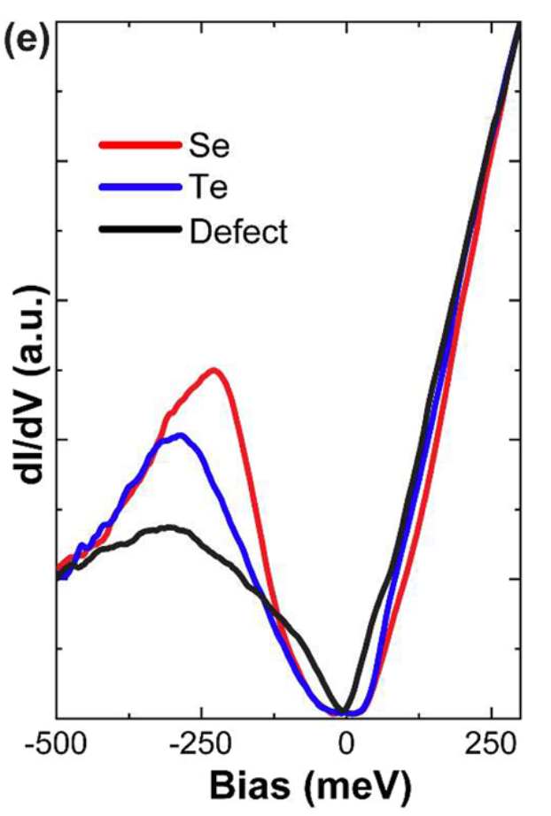
Fe(Se, S) / FeSe
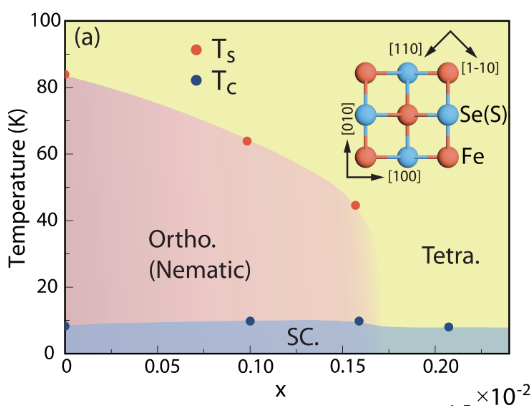
FeSe is a prototypical s$^{\pm}$-wave superconductor with electronic nematicity and orbital-selective Cooper pairing preferentially from the $d_{yz}$ orbitals of Fe.
It is observed that the linear relationship Eq. ((eq:linearrelationship)) is broken in Nb-FeSe spectrum, this indicates the Josephson current in this case is adjusted due to phase difference in $s^{\pm}$ orbitals.
In Fe (Se, S), the nameticity order has a complex computing relationship with the superconductivity order. The namaticity order in FeSe and low doping phase of FeSeS makes Fe-1 and Fe-2 asymmetry, which means an intra-cell broken symmetry, from $C_4$ to $C_2$. More detailed, for FeSe$_{1-x}$S$_x$ [@hanaguri_two_2018]:
$x<0.17$, the phase is called nematicity phase, which is anisotropic. In this phase, the electronically driven nematic phase causes the lifting degeneracy between $d_{xz}$ and $d_{yz}$ orbitals. The orbital order rearanges the electrons and enhances the pairing respectively, leading to 3 gaps: $\pm0.6$meV (mainly electron-like d${xy}$ band), $\pm 2.5$meV (mainly hole-like $d{yz}$ band located at the hole band at $\Gamma$ point), and $\pm4.0$meV (mainly hole-like $d_{xz}$ band). It has reported that an extra gap 1.3meV at M point, contributed by an electon band.
$x=0.17$, nematicity end poing (NEP).
$x>0.17$, Nematic order disappears. Electrons are isotropic and the $d_{xz}$ and $d_{yz}$ orbitals are degenerated, weaken the pairing mechanism as the two orbitals are suggested can not conduct pairing interactions simultaneously. The superconducting gap shrinks with increasing $x$.
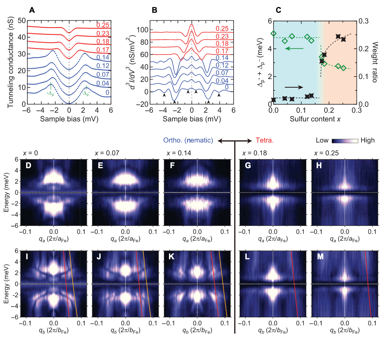
BQPI analysis
There is convinced that strong BQPI occurs in electron pocket centered at M point, which can be seen from FFT of $g(r,V=0.6meV)$.
Pair Density Waves
Review the Eq. ((eq:CooperEnergy)), under an infinitesimal attractive potential the electrons above the FS and below the Debye frequency tend to form pairs, which has zero momentum at all. However, the emergent unconventional superconducting phenomenon indicates the potential opposition of this statement. Fulde-Ferrell-Larkin-Ovchinnikov (FFLO) state is predicted by breaking of time-reversal symmetry in a superconducting state by a Zeeman magnetic field, finite momentum pairing.
Pair density wave state is a superconducting state without Zeeman magnetic field with spatially modulated order parameter.
Phase Field and Drift Field
For an ideal 2D lattice, wisely choosing the root coordinates, the distribution field should be: \(A(\mathbf r)=A_1(\mathbf{r})\cos(\mathbf{Q}_1\cdot\mathbf{r})+A_2(\mathbf{r})\cos(\mathbf{Q}_2\cdot\mathbf{r})\) The drift will introduce a extra low-frequency field $u(\mathbf{r})$: $\mathbf{r}\to\mathbf{r}+u(\mathbf{r})$. The resulting topograph is: \(\begin{split} A(\mathbf{r}) &= A_1(\mathbf{r})\cos\{\mathbf{Q_x}\cdot(\mathbf{r}+\mathbf{u}(\mathbf{r}))\}+A_2(\mathbf{r})\cos\{\mathbf{Q_y}\cdot(\mathbf{r}+\mathbf{u}(\mathbf{r}))\} \\ &= A_1(\mathbf{r})\cos\{(\mathbf{Q_x}\cdot\mathbf{r})+(\mathbf{Q_x}\cdot\mathbf{u}(\mathbf{r}))\}+A_2(\mathbf{r})\cos\{(\mathbf{Q_y}\cdot(\mathbf{r})+(\mathbf{Q_x}\cdot\mathbf{u}(\mathbf{r}))\} \\ &= A_1(\mathbf{r})\cos(\mathbf{Q_x}\cdot\mathbf{r} + \phi_x) + A_2(\mathbf{r})\cos(\mathbf{Q_y}\cdot\mathbf{r} + \phi_y) \end{split}\) The lock-in measurement is based on Fourier transformation and gaussion mask. For the $\mathbf Q_x$ modulated part: Take $A(\vec{r}) = cos{\vec{Q_x}\cdot\vec{r} + \phi_x}$ as an example. We will construct two sets of lock-in reference with wavevectors $\vec{Q_x}$ and $\vec{Q_y}$
since $cos(\vec{Q_x}\cdot\vec{r} + \phi_x) = cos(\vec{Q_x}\cdot\vec{r})cos(\phi_x)-sin(\vec{Q_x}\cdot\vec{r})sin(\phi_x)$
\[\begin{cases} A_{xx} = A \times cos(\vec{Q_x}\cdot\vec{r}) = cos^2(\vec{Q_x}\cdot\vec{r})cos(\phi_x)-sin(\vec{Q_x}\cdot\vec{r})cos(\vec{Q_x}\cdot\vec{r})sin(\phi_x)\\ A_{xy} = A \times sin(\vec{Q_x}\cdot\vec{r}) = sin(\vec{Q_x}\cdot\vec{r})cos(\vec{Q_x}\cdot\vec{r})cos(\phi_x)-sin^2(\vec{Q_x}\cdot\vec{r})sin(\phi_x) \end{cases}\]that is,
\[\begin{cases} A_{xx} = \frac{1}{2}\{1+cos(2\vec{Q_x}\cdot\vec{r})\}cos(\phi_x)-sin(\vec{Q_x}\cdot\vec{r})cos(\vec{Q_x}\cdot\vec{r})sin(\phi_x)\\ A_{xy} = sin(\vec{Q_x}\cdot\vec{r})cos(\vec{Q_x}\cdot\vec{r})cos(\phi_x)-\frac{1}{2}\{1-sin(2\vec{Q_x}\cdot\vec{r}))\}sin(\phi_x) \end{cases}\]When applying a gaussian low-pass filter $g = \frac{1}{\sqrt{2\pi}\sigma_q}e^{\frac{q^2}{2\sigma_q^2}}$, the modulations with frequency exceed $\frac{2\pi}{\sigma_q}$ will be suppressed. Set $\frac{2\pi}{\sigma_q}<Q_x$, the oscillation parts will be smeared and the phase field remains: \(\begin{cases} F^{-1}(g\cdot F(A_{xx})) = \frac{1}{2}cos(\phi_x)\\ F^{-1}(g\cdot F(A_{xy})) = -\frac{1}{2}sin(\phi_x)\\ \end{cases}\)
The generalized/complex form of the 2 dimensional lock-in method can be implemented as: \(A_\mathbf{Q}(\boldsymbol{r})=\mathcal{F}^{-1}A_\mathbf{Q}(\boldsymbol{q})=\mathcal{F}^{-1}\left\{\mathcal{F}\left[A(\boldsymbol{r})\mathrm{e}^{\mathrm{i}\mathbf{Q}\cdot\boldsymbol{r}}\right]\cdot\frac{1}{\sqrt{2\pi}\sigma_\mathrm{q}}\mathrm{e}^{-\frac{q^2}{2{\sigma_\mathrm{q}}^2}}\right\}\) This is actually equal to the form: \(A_\mathbf{Q}(\boldsymbol{r})=\int\mathrm{d}\boldsymbol{R}A(\boldsymbol{R})\mathrm{~e}^{i\mathbf{Q}\cdot\boldsymbol{R}}\mathrm{~e}^{-\frac{(\boldsymbol{r}-\boldsymbol{R})^2}{2\sigma^2}}\) Since the Fourier transformation of Gaussian is still Gaussian. The Gaussian factor plays a role like Window. The second integration is just a Window Fourier Transformation.
Pair Breaking Scattering Inteference
Starting from BdG Hamiltonian: \(H_{BdG}=\sum_{\mathbf{k}}\Psi_{\mathbf{k}}^{\dagger}\begin{pmatrix}\xi_{\mathbf{k}}&\Delta_{\mathbf{k}}\\\Delta_{\mathbf{k}}^{*}&-\xi_{\mathbf{k}}\end{pmatrix}\Psi_{\mathbf{k}}\) Assume the scattering occurs between two hot spots $\mathbf{k}1$ and $\mathbf{k}_2$ under the same ergodic surface. $\varepsilon_k=0$, which is based on the small pairing energy gap and a flat band corresponding to the large DOS. And we focused on the sign-changing scattering: $\Delta{\mathbf{k}1}=\Delta_0,\Delta{\mathbf{k}2}=-\Delta_0$. When there is no impurities, the eigenfunction $H\phi=\Delta_0\phi$ gives: \(\begin{align} \mathbf{k}_1:&\begin{pmatrix}0&\Delta_0\\\Delta_0&0\end{pmatrix}\begin{pmatrix}u_1\\v_1\end{pmatrix}=\Delta_0\begin{pmatrix}u_1\\v_1\end{pmatrix}\Longrightarrow u_1=v_1\\ \mathbf{k}_2:&\begin{pmatrix}0&&-\Delta_0\\-\Delta_0&&0\end{pmatrix}\begin{pmatrix}u_2\\v_2\end{pmatrix}=\Delta_0\begin{pmatrix}u_2\\v_2\end{pmatrix}\mathrm{~}\Longrightarrow\mathrm{~}-\Delta_0v_2=\Delta_0u_2\mathrm{~}\Longrightarrow\mathrm{~}u_2=-v_2 \end{align}\) For a scalar impurity potential inducing the scattering, the potential can be expressed as $\equiv V\tau{z}$. Projecting into the subspace spanned by ${\phi_1,\phi_2}$: \(M_{12}=\langle\phi_1|V\tau_z|\phi_2\rangle=\frac{V}{2}\begin{pmatrix}1&1\end{pmatrix}\begin{pmatrix}1&0\\0&-1\end{pmatrix}\begin{pmatrix}1\\-1\end{pmatrix}=\frac{V}{2}\begin{pmatrix}1&1\end{pmatrix}\begin{pmatrix}1\\1\end{pmatrix}=V=M_{21}\)2 The full Hamiltonian is: \(H_{eff}=\begin{pmatrix}\Delta_0&V\\V&\Delta_0\end{pmatrix}\Rightarrow E_\pm=\Delta_0\pm V\) The eigenvectors are the symmetric and asymmetrc composition of ${\phi_1,\phi_2}$: \(\begin{align} \Psi_{L}(\mathbf{r})&=\frac{1}{\sqrt{2}}[\phi_{1}(\mathbf{r})+\phi_{2}(\mathbf{r})]=\frac{1}{2}\left[\begin{pmatrix}1\\1\end{pmatrix}e^{i\mathbf{k}_{1}\cdot\mathbf{r}}+\begin{pmatrix}1\\-1\end{pmatrix}e^{i\mathbf{k}_{2}\cdot\mathbf{r}}\right]\\ &u_L(\mathbf{r})=\frac{1}{2}(e^{i\mathbf{k}_1\cdot\mathbf{r}}+e^{i\mathbf{k}_2\cdot\mathbf{r}}),v_L(\mathbf{r})=\frac{1}{2}(e^{i\mathbf{k}_1\cdot\mathbf{r}}-e^{i\mathbf{k}_2\cdot\mathbf{r}})\\ \Psi_{S}(\mathbf{r})&=\frac{1}{\sqrt{2}}[\phi_{1}(\mathbf{r})-\phi_{2}(\mathbf{r})]=\frac{1}{2}\left[\begin{pmatrix}1\\1\end{pmatrix}e^{i\mathbf{k}_{1}\cdot\mathbf{r}}-\begin{pmatrix}1\\-1\end{pmatrix}e^{i\mathbf{k}_{2}\cdot\mathbf{r}}\right]\\ &u_S(\mathbf{r})=\frac{1}{2}(e^{i\mathbf{k}_1\cdot\mathbf{r}}-e^{i\mathbf{k}_2\cdot\mathbf{r}}),v_S(\mathbf{r})=\frac{1}{2}(e^{i\mathbf{k}_1\cdot\mathbf{r}}+e^{i\mathbf{k}_2\cdot\mathbf{r}}) \end{align}\) In negative bias, the wavefunction is contributed by the electronic component: \(\begin{align} -\Delta_L: P_{-\Delta_L}^e=|u|^2\propto|1+e^{-i\mathbf{q}\cdot\mathbf{r}}|^2\propto1+\cos(\mathbf{q}\cdot\mathbf{r})\\ -\Delta_S: P_{-\Delta_S}^e=|u|^2\propto|1-e^{-i\mathbf{q}\cdot\mathbf{r}}|^2\propto1-\cos(\mathbf{q}\cdot\mathbf{r}) \end{align}\) Positive bias: \(\begin{align} \Delta_L: P_{\Delta_L}^h=|v|^2\propto1-\cos(\mathbf{q}\cdot\mathbf{r})\\ \Delta_S: P_{\Delta_S}^h=|v|^2\propto1+\cos(\mathbf{q}\cdot\mathbf{r}) \end{align}\) The LDOS is: \(L(E+\Delta_{L})+[1-\cos(\mathbf{q}\cdot\mathbf{r})]L(E+\Delta_{S})+[1-\cos(\mathbf{q}\cdot\mathbf{r})]L(E-\Delta_L)+[1+\cos(\mathbf{q}\cdot\mathbf{r})]L(E-\Delta_S)\)
Green function method {#green-function-method .unnumbered}
From the wavefunction to quasi-particle interference (QPI) analysis, we need the Green function.
The unperturbed propagator of SC quasi-particle in Nambu basis is: \(G_0(\mathbf{k},\omega)=\frac{1}{\omega^2-E_{\mathbf{k}}^2}\begin{pmatrix}\omega+\xi_{\mathbf{k}}&\Delta_{\mathbf{k}}\\\Delta_{\mathbf{k}}&\omega-\xi_{\mathbf{k}}\end{pmatrix}\) where $E_{\mathbf{k}}=\sqrt{\xi_{\mathbf{k}}^2+\Delta_{\mathbf{k}}^2}$. Introducing an impurity potential $V\tau_z$ like above, the modified propagator is leaded by: \(\delta G(\mathbf{k},\mathbf{k}^{\prime},\omega)\approx G_0(\mathbf{k},\omega)\hat{V}G_0(\mathbf{k}^{\prime},\omega)\) The (1,1) element of the propagator is proportional to $\braket{c c^\dagger}$, which is the propagator of electrons and able to be seen by STS. Calculations show: \(\delta G(\mathbf{k},\mathbf{k}^{\prime},\omega)_{(1,1)}\propto(\omega+\xi)(\omega+\xi^{\prime})-\Delta\Delta^{\prime}\) We have known that: \(\begin{aligned}u_{\mathbf{k}}^{2}&=\frac{1}{2}\left(1+\frac{\xi_{\mathbf{k}}}{E_{\mathbf{k}}}\right),\quad v_{\mathbf{k}}^{2}=\frac{1}{2}\left(1-\frac{\xi_{\mathbf{k}}}{E_{\mathbf{k}}}\right)\\&u_{\mathbf{k}}v_{\mathbf{k}}=\frac{\Delta_{\mathbf{k}}}{2E_{\mathbf{k}}}\end{aligned}\) Then: \(\begin{align} (\omega+\xi)(\omega+\xi^{\prime})-\Delta\Delta^{\prime}&=(2Eu^2)(2E^{\prime}u^{\prime2})-(2Euv)(2E^{\prime}u^{\prime}v^{\prime})\\ &=4EE^{\prime}\cdot uu^{\prime}\cdot(uu^{\prime}-vv^{\prime}) \end{align}\) The denominator of the Green function is: \(\frac{1}{\omega^2-E^2}\approx\frac{1}{2E(\omega-E)},\omega\to E\) Multiply them (notice the denominator enters as square) : \(\begin{align}\mathrm{QPI~Signal}&\propto\frac{\mathrm{Numerator}}{\text{Denominator}}=\frac{4EE^{\prime}\cdot uu^{\prime}(uu^{\prime}-vv^{\prime})}{4EE^{\prime}}\\&\Longrightarrow\mathrm{~u_ku_{k^{\prime}}(u_ku_{k^{\prime}}-v_kv_{k^{\prime}})}\end{align}\) If sign-changing happens, like what showing before $v_k=-v_{k’}$, the inteference is enhanced. [($\clubsuit$ TODO: The formal and complete analysis should look into reference [@hirschfeld_robust_2016] $\clubsuit$)]{style=”color: OliveGreen”}
PR-QPI
Group Theory Application in STM topograph
The Group Definition
The technique can decompose the LDOS into different fourier components. The complex number set ${\mathbf{A}(\mathbf{Q}_i,\mathbf{r})}$ can be viewed as a vector space $V$, the all mapping $V\to V$, in orther words, the symmetric actions on the space $V$ form a group $G$.
As space $V$ is has momentum index $Q$ and position index $r$ at the same time, it is the combination of translation and rotation: \(g:A(Q_i,r)\mapsto A(Q_j,g\cdot r)\times e^{i\delta Q\cdot \delta r}\) The whole group is called Space Group $\mathscr S$. Just like the expression of the group element, the whole group is the direct product of the two subgroup, Point Group $\mathscr P$ and Translation Group $\mathscr T$. The relation between them is: \(\mathscr P = \mathscr S/\mathscr T\) In lattice the momentum vector $b$, or so-called reciprocal vector has the properties: \(b_i\cdot a_j=2\pi \delta_{ij}\) Then if we focused on the LDOS peaked at $b_i$, the phase vanished, which means the whole space group $\mathscr S$ is reduced to the point group $\mathscr P$. However, if target $Q$ is rationable multiple to reciprocal vector, we can reform a super-lattice based on a multiple of original reciprocal vectors. The new basis of reciprocal vectors form a new translation group $\mathscr T’$, which reform the Point group into Extended Point Group $\mathscr P’=\mathscr S/\mathscr T’$.
Example: Triple-$Q$ Commensurate Charge Density Wave in 2H–NbSe$_2$ {#example-triple-q-commensurate-charge-density-wave-in-2hnbse_2 .unnumbered}
A concrete example of a commensurate modulation with finite wavevector is provided by the triple-$Q$ charge density wave (CDW) observed in transition-metal dichalcogenides such as 2H–NbSe$_2$ and 2H–TaSe$_2$.
Underlying lattice.
The parent crystal is a hexagonal lattice with primitive translation vectors $\mathbf{a}1, \mathbf{a}_2$, and point group symmetry $D{6h}$. The reciprocal lattice is generated by the corresponding vectors $\mathbf{b}_1, \mathbf{b}_2$.
Modulation wavevectors.
At low temperatures, the system develops a commensurate CDW characterized by three ordering wavevectors at the Brillouin zone boundary: \(\mathbf{Q}_1 = \tfrac{1}{3}\mathbf{b}_1, \quad \mathbf{Q}_2 = \tfrac{1}{3}\mathbf{b}_2, \quad \mathbf{Q}_3 = -\tfrac{1}{3}(\mathbf{b}_1 + \mathbf{b}_2).\) Each $\mathbf{Q}_i$ is a rational fraction of a reciprocal lattice vector, so the CDW is commensurate.
Enlarged unit cell.
The CDW triples the real-space periodicity, giving rise to a new $3 \times 3$ supercell. The original translation group $T$, generated by $\mathbf{a}_1, \mathbf{a}_2$, is reduced to a subgroup $T_f$, generated by $3\mathbf{a}_1, 3\mathbf{a}_2$. Translations by $\mathbf{a}_1$ or $\mathbf{a}_2$ no longer leave the CDW invariant, but translations by $3\mathbf{a}_1$ or $3\mathbf{a}_2$ do.
Extended point group.
The space group $S$ of the parent lattice can be factorized as $\mathscr S = \mathscr T \otimes \mathscr P$, where $\mathscr P$ is the point group. In the CDW phase, one considers instead the factor group \(\mathscr P_e = \mathscr S / \mathscr T_f,\) which is the extended point group associated with the enlarged translation subgroup $\mathscr T_f$. Elements of the original translation group that are no longer symmetries of the CDW (such as $\mathbf{a}_1$) appear as new elements of the extended point group. Thus, the CDW order can be classified by irreducible representations of $G_e$, effectively treating the commensurate finite-$Q$ order as if it were a $\Gamma$-point order parameter in the folded Brillouin zone.
Physical manifestation.
In scanning tunneling microscopy (STM), the local density of states (LDOS) exhibits both the atomic-scale periodicity of the underlying lattice and the longer $3 \times 3$ modulation pattern of the CDW. Fourier analysis reveals peaks at the commensurate wavevectors $\mathbf{Q}_i$. Because these are folded to the new Brillouin zone center, the LDOS modulations can be decomposed into symmetry-distinct components according to the irreducible representations of the extended point group $G_e$.
Group Theory Application
Now suppose we have constructed the extended point group $\Tilde{\mathscr P}$, it can be redusible. An irreducible representations (irreps.) of $\Tilde{\mathscr P}$ is denoted as $\Gamma$, its degeneracy/multiplicity is: \(n_\Gamma=\frac{1}{|\mathscr{G}|}\sum_{g\in\widetilde{\mathscr{G}}}\chi_\Gamma(g)\chi(g)\) Then the reps. of $\Tilde{\mathscr P}$ can be decomposed into the direct sum of irreps.: \(D(g)\cong\bigoplus_\Gamma n_\Gamma D^\Gamma(g),\) Because of the orthonomality of the irreps. \(\frac{1}{|G|}\sum_{g\in G}\chi_\Gamma^*(g)\chi_{\Gamma^{\prime}}(g)=\delta_{\Gamma,\Gamma^{\prime}}.\) We can use the orthogonalization method to build the basis of the irreps.: \(\mathcal{P}_\Gamma=\frac{d_\Gamma}{|G|}\sum_{g\in G}\chi_\Gamma^*(g)D(g),\) In our LDOS anaylsis, the irreps. is often real and 1 dimensional. So the simplified projection operator is: \(\mathcal{P}_\Gamma=\frac{1}{\left|\mathcal{G}\right|}\sum_{g\in\widetilde{\mathscr{G}}}\chi_\Gamma(g)g\)
Symmetry properties at different levels {#symmetry-properties-at-different-levels .unnumbered}
1. Hamiltonian $H$.
The Hamiltonian encodes the full microscopic description of the system (lattice, interactions, potentials). It is invariant under the full symmetry group $S$, which may include translations, point group operations, and internal symmetries. This is the “parent” symmetry that constrains all possible eigenstates.
2. Wavefunction $\Psi_k(\mathbf r)$.
Each eigenstate of $H$ transforms according to an irreducible representation (irrep) of $S$. A wavefunction does not realize the entire group structure, but instead provides one specific realization of an irrep.
3. Local density of states (LDOS).
\[\mathrm{LDOS}(\mathbf r, E) = \sum_k |\Psi_k(\mathbf r)|^2 \, \delta(E_k - E) .\]In the absence of symmetry breaking, the LDOS transforms as the trivial irrep of $S$.
When an order parameter is present, the system’s symmetry is reduced from $S$ to a subgroup $S’$. In this case the LDOS must transform trivially under $S’$, but may decompose into non-trivial irreps of the original group $S$. This decomposition reveals which symmetries have been broken.
4. STM measurement.
The scanning tunneling microscope (STM) measures the tunneling current, which is directly proportional to the LDOS: \(I(\mathbf r, E) \propto \mathrm{LDOS}(\mathbf r, E).\) Thus STM inherits the symmetry of the LDOS (possibly further reduced by surface effects). STM therefore acts as a direct probe of symmetry breaking in real space.
Summary:
The Hamiltonian has the largest symmetry (full group $S$).
Wavefunctions transform as irreps of $S$.
The LDOS is trivial under $S$ if unbroken, but symmetry breaking reduces invariance to $S’$ and reveals non-trivial irreps.
STM detects exactly this LDOS symmetry, making it an experimental window into order parameters and broken symmetries.
When order parameter is zero, the symmetry of the LDOS is the whole symmetry of the system, $\mathscr S$.LDOS is trivial under all irreps. of $\mathscr S$, which means: \(\forall g \in \mathscr S, g\cdot LDOS(Q,r)=LDOS(Q,r)\Leftrightarrow D(g)=1\). When symmetry breaks and order parameter emerges, one or some of the irreps. related with the broken symmetry is no longer the subgroups of the symmetry group, thus $\mathscr S$ is degraded to a smaller group $\mathscr S’$, consisting with all preserved symmetries. The irreps. in $\mathscr S’$ is still trivial, but the extra symmetry in $\mathscr S$ is non-trivial, which signals the order parameter.
This can be seen in Clifford Algebra, in which the properties of the geometric product lead to the anti-commutation of $\gamma$. See in Dirac matrices and Clifford Algebra and Geometric Algebra ↩
It can be seen here if pairing has the same sign, the matrix element will be zero. Actually the Anderson’s Theorem which claims that the SC gap is protected from the non-magnetic impurity. ↩